Unsupervised learning: \(k\)-means clustering

SURE 2025

Department of Statistics & Data Science
Carnegie Mellon University

Background

Recap: Unsupervised learning

• In unsupervised learning, we are only given a (big) data matrix that are not labeled

• Dimension reduction: Can we meaningfully reduce the dimension of the data either so we can visualize it?

• PCA answers this questions by finding “interesting directions” and projecting the data on to those directions

• Besides dimension reduction, clustering is another fundamental problem in unsupervised learning

Clustering (cluster analysis)

Clustering refers to a very broad set of techniques for finding subgroups, or clusters, in a data set — ISLR

Goals: partition of the observations into distinct clusters so that

• observations within clusters are more similar to each other

• observations in different clusters are more different from each other

• This often involves domain-specific considerations based on knowledge of the provided data

• Besides tabular data, clustering can be applied to other types of data (e.g., curves/functions, shapes, graphs/networks, images, etc.)

Types of clustering

• Hard clustering (\(k\)-means, hierarchical)

  • output hard assignments

  • strictly assign observations to only one cluster

• Soft/fuzzy clustering (model-based clustering, mixture model)

  • output soft assignments

  • assign an observation a probability of belonging to each cluster

  • provide uncertainty in the clustering results

  • incorporate statistical modeling into clustering

Distance between observations

• What does it means for two or more observations to be similar or different?

• This require characterizing the distance between observations

  • Clusters: groups of observations that are “close” together

• This is easy to do for 2 quantitative variables: just make a scatterplot

But how do we define “distance” beyond 2D data?

Let \(\boldsymbol{x}_i = (x_{i1}, \dots, x_{ip})\) be a vector of \(p\) features for observation \(i\)

Question of interest: How “far away” is \(\boldsymbol{x}_i\) from \(\boldsymbol{x}_j\)?

When looking at a scatterplot, we’re using Euclidean distance \[d(\boldsymbol{x}_i, \boldsymbol{x}_j) = \sqrt{(x_{i1} - x_{j1})^2 + \dots + (x_{ip} - x_{jp})^2}\]

Distances in general

• There’s a variety of different types of distance metrics: Manhattan, Mahalanobis, Cosine, Kullback-Leibler, Hellinger, Wasserstein

• We’re just going to focus on Euclidean distance

• Let \(d(\boldsymbol{x}_i, \boldsymbol{x}_j)\) denote the pairwise distance between two observations \(i\) and \(j\)

1. Identity: \(\boldsymbol{x}_i = \boldsymbol{x}_j \Leftrightarrow d(\boldsymbol{x}_i, \boldsymbol{x}_j) = 0\)

2. Non-negativity: \(d(\boldsymbol{x}_i, \boldsymbol{x}_j) \geq 0\)

3. Symmetry: \(d(\boldsymbol{x}_i, \boldsymbol{x}_j) = d(\boldsymbol{x}_j, \boldsymbol{x}_i)\)

4. Triangle inequality: \(d(\boldsymbol{x}_i, \boldsymbol{x}_j) \leq d(\boldsymbol{x}_i, \boldsymbol{x}_k) + d(\boldsymbol{x}_k, \boldsymbol{x}_j)\)

Distance Matrix: matrix \(D\) of all pairwise distances

• \(D_{ij} = d(\boldsymbol{x}_i, \boldsymbol{x}_j)\)

• where \(D_{ii} = 0\) and \(D_{ij} = D_{ji}\)

\[D = \begin{pmatrix} 0 & D_{12} & \cdots & D_{1n} \\ D_{21} & 0 & \cdots & D_{2n} \\ \vdots & \vdots & \ddots & \vdots \\ D_{n1} & \cdots & \cdots & 0 \end{pmatrix}\]

Units matter in clustering

• Variables are typically measured in different units

• One variable may dominate others when computing Euclidean distance because its range is much larger

• Scaling of the variables matters!

• Standardize each variable in the dataset to have mean 0 and standard deviation 1 with scale()

\(k\)-means clustering

\(k\)-means clustering

• Goal: partition the observations into a pre-specified number of clusters

• Idea behind \(k\)-means clustering: a “good” clustering is one for which the within-cluster variation is as small as possible

• We want to minimize the within-cluster variation \(W(C_k)\) for each cluster \(C_k\) (i.e. the amount by which the observations within a cluster differ from each other)

• This is equivalent to solving \(\qquad \underset{C_1, \dots, C_K}{\text{minimize }} \Big\{ \sum_{k=1}^K W(C_k) \Big\}\)

• In words, we want to

  • partition the observations into \(k\) clusters

  • so that the total within-cluster variation, summed over all \(k\) clusters, is as small as possible

• Keep in mind… the clusters are non-overlapping: no observation belongs to more than 1 cluster

\(k\)-means clustering

How do we define within-cluster variation?

• Use the (squared) Euclidean distance \[W(C_k) = \frac{1}{|C_k|}\sum_{i,j \in C_k} d(x_i, x_j)^2 \,,\] where \(|C_k|\) denote the number of observations in cluster \(k\)

• Commonly referred to as the within-cluster sum of squares (WSS)

So how do we solve this?

Lloyd’s algorithm (naive \(k\)-means)

Watch this video

• Input: the value for \(k\)

• Initialization: randomly choose \(k\) centroids (i.e. \(k\) means).

• Proceed by alternating between two steps

  1. Assignment step: assign each observation to the cluster with the nearest centroid (using Euclidean distance)

  2. Update step: compute new centroids as the averages of the updated groups & reassign each observations to closest centroid

• Repeat until cluster assignment stop changing

Some notes on the algorithm

• The algorithm starts from a random initialization, hence results will change from run to run (set the seed!)

• We’re not guaranteed to find the global optimum of its objective function (WSS); instead it typically converges to a local optimum

• We will attempt to fix randomness issue later

Watch this video

Gapminder data

Health and income outcomes for 184 countries from 1960 to 2016 from the famous Gapminder project

library(tidyverse)
theme_set(theme_light())
library(dslabs)
glimpse(gapminder)

Rows: 10,545
Columns: 9
$ country          <fct> "Albania", "Algeria", "Angola", "Antigua and Barbuda"…
$ year             <int> 1960, 1960, 1960, 1960, 1960, 1960, 1960, 1960, 1960,…
$ infant_mortality <dbl> 115.40, 148.20, 208.00, NA, 59.87, NA, NA, 20.30, 37.…
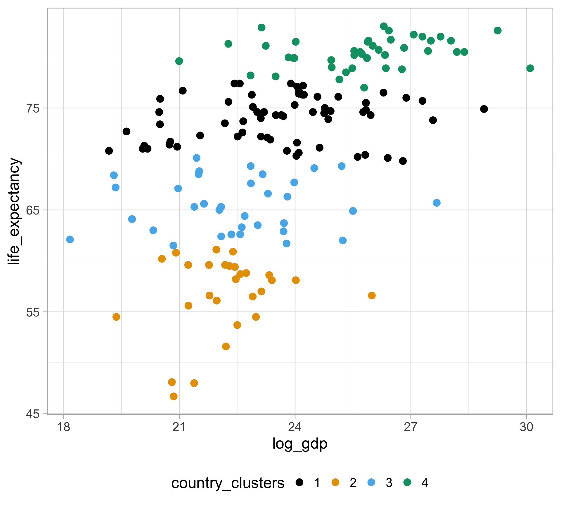
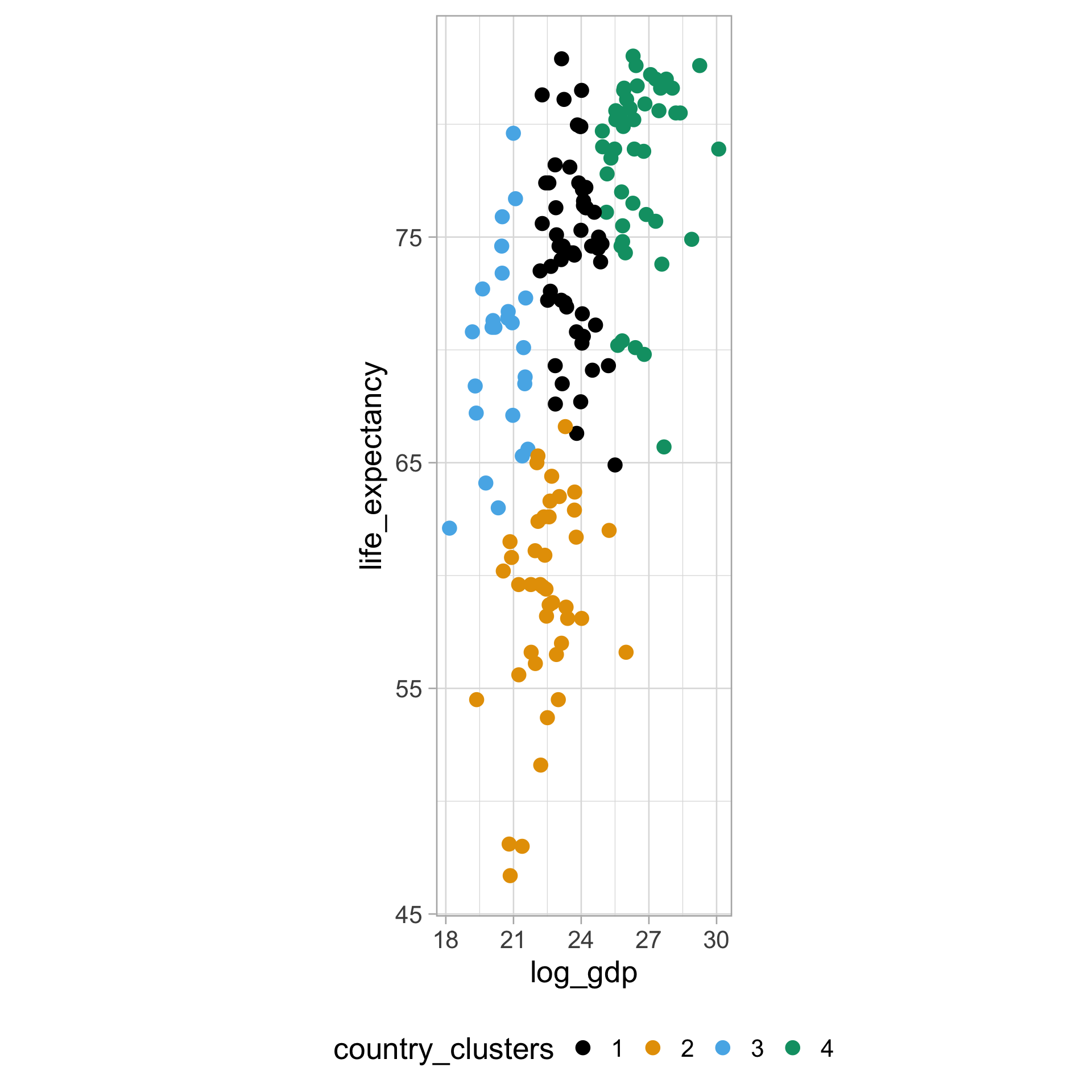
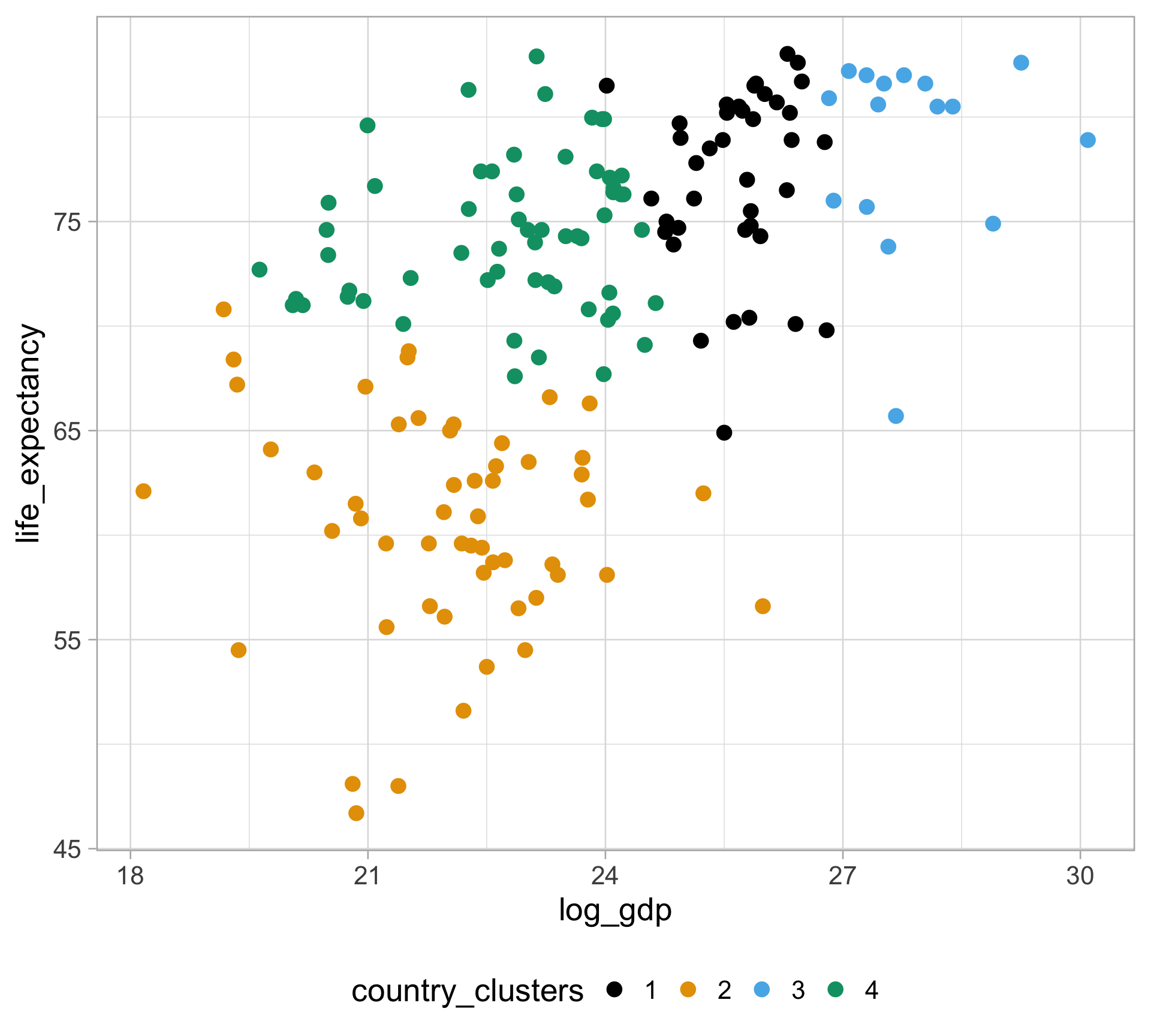
$ life_expectancy  <dbl> 62.87, 47.50, 35.98, 62.97, 65.39, 66.86, 65.66, 70.8…
$ fertility        <dbl> 6.19, 7.65, 7.32, 4.43, 3.11, 4.55, 4.82, 3.45, 2.70,…
$ population       <dbl> 1636054, 11124892, 5270844, 54681, 20619075, 1867396,…
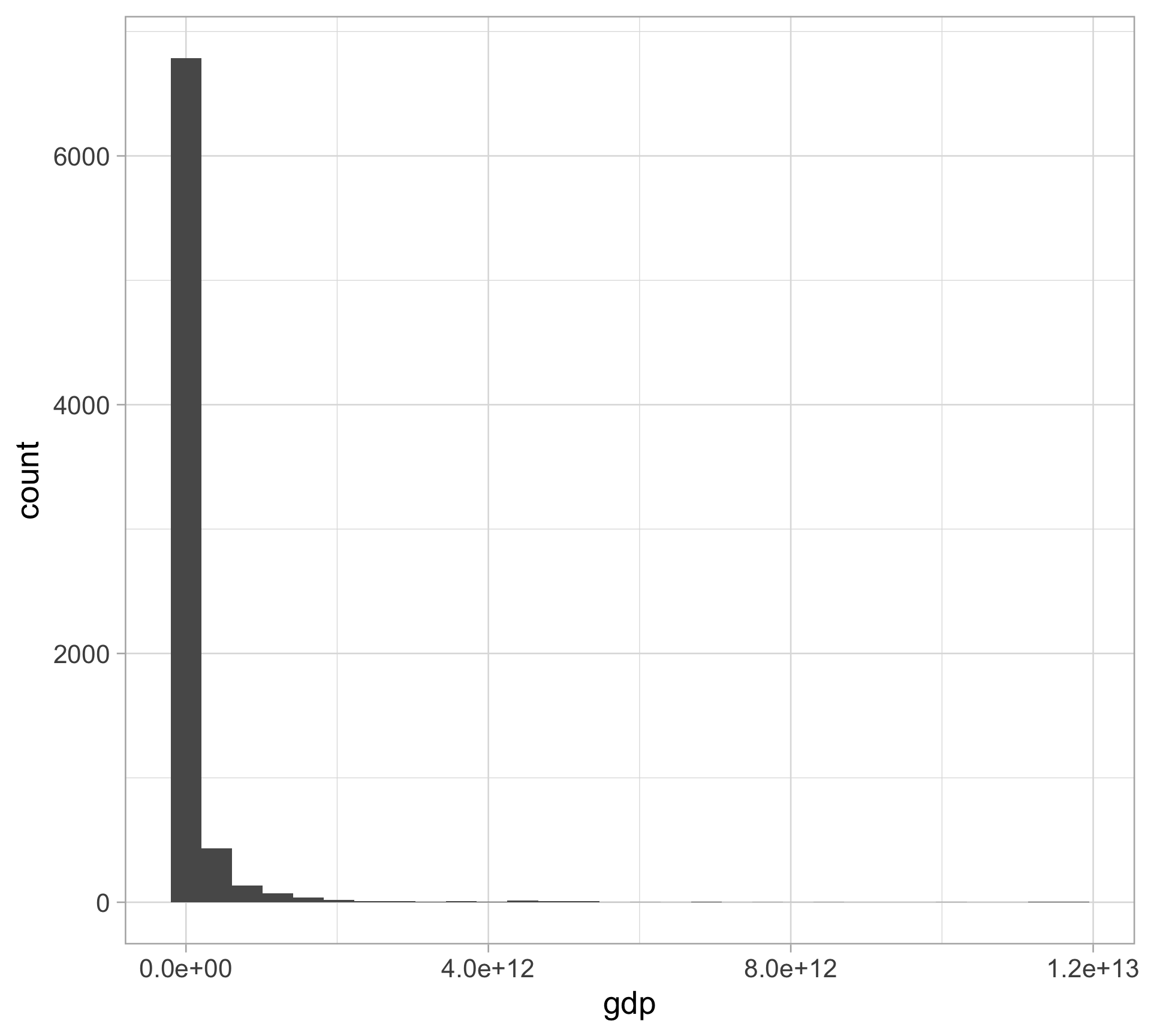
$ gdp              <dbl> NA, 13828152297, NA, NA, 108322326649, NA, NA, 966778…
$ continent        <fct> Europe, Africa, Africa, Americas, Americas, Asia, Ame…
$ region           <fct> Southern Europe, Northern Africa, Middle Africa, Cari…

GDP is severely skewed right…

gapminder |> 
  ggplot(aes(x = gdp)) + 
  geom_histogram() 

Some initial cleaning…

• Each row is at the country-year level

• Focus on data for 2011 where gdp is not missing

• Log-transform gdp

clean_gapminder <- gapminder |>
  filter(year == 2011, !is.na(gdp)) |>
  mutate(log_gdp = log(gdp))

\(k\)-means clustering example

Note: only 2 features are used in this example (gdp and life_expectancy),
but in practice, you can (should) include more than two features

• Use the kmeans() function, but must provide number of clusters \(k\)

init_kmeans <- clean_gapminder |> 
  select(log_gdp, life_expectancy) |> 
  kmeans(algorithm = "Lloyd", centers = 4, nstart = 1)

clean_gapminder |>
  mutate(
    country_clusters = as.factor(init_kmeans$cluster)
  ) |>
  ggplot(aes(x = log_gdp, y = life_expectancy,
             color = country_clusters)) +
  geom_point(size = 4) + 
  ggthemes::scale_color_colorblind() +
  theme(legend.position = "bottom") 

Careful with units…

• Use coord_fixed() so that the axes match with unit scales

clean_gapminder |>
  mutate(
    country_clusters = as.factor(init_kmeans$cluster)
  ) |>
  ggplot(aes(x = log_gdp, y = life_expectancy,
             color = country_clusters)) +
  geom_point(size = 4) + 
  ggthemes::scale_color_colorblind() +
  theme(legend.position = "bottom") +
  coord_fixed()

Standardize the variables!

• Use the scale() function to first standardize the variables, \(\frac{\text{value} - \text{mean}}{\text{sd}}\)

clean_gapminder <- clean_gapminder |>
  mutate(
    std_log_gdp = as.numeric(scale(log_gdp, center = TRUE, scale = TRUE)),
    std_life_exp = as.numeric(scale(life_expectancy, center = TRUE, scale = TRUE))
  )

std_kmeans <- clean_gapminder |> 
  select(std_log_gdp, std_life_exp) |> 
  kmeans(algorithm = "Lloyd", centers = 4, nstart = 1)

clean_gapminder |>
  mutate(
    country_clusters = as.factor(std_kmeans$cluster)
  ) |>
  ggplot(aes(x = log_gdp, y = life_expectancy,
             color = country_clusters)) +
  geom_point(size = 4) + 
  ggthemes::scale_color_colorblind() +
  theme(legend.position = "bottom") +
  coord_fixed()

Standardize the variables!

clean_gapminder |>
  mutate(
    country_clusters = as.factor(std_kmeans$cluster)
  ) |>
  ggplot(aes(x = std_log_gdp, y = std_life_exp,
             color = country_clusters)) +
  geom_point(size = 4) + 
  ggthemes::scale_color_colorblind() +
  theme(legend.position = "bottom") +
  coord_fixed()

And if we run it again?

We get different clustering results!

another_kmeans <- clean_gapminder |> 
  select(std_log_gdp, std_life_exp) |> 
  kmeans(algorithm = "Lloyd", centers = 4, nstart = 1)

clean_gapminder |>
  mutate(
    country_clusters = as.factor(another_kmeans$cluster)
  ) |>
  ggplot(aes(x = log_gdp, y = life_expectancy,
             color = country_clusters)) +
  geom_point(size = 4) + 
  ggthemes::scale_color_colorblind() +
  theme(legend.position = "bottom")

Results depend on initialization

Keep in mind: the labels / colors are arbitrary

Fix randomness issue with nstart

Run the algorithm nstart times, then pick the results with lowest total within-cluster variation \[\text{total WSS} = \sum_{k=1}^K W(C_k)\]

nstart_kmeans <- clean_gapminder |> 
  select(std_log_gdp, std_life_exp) |> 
  kmeans(algorithm = "Lloyd", centers = 4, nstart = 30)

clean_gapminder |>
  mutate(
    country_clusters = as.factor(nstart_kmeans$cluster)
  ) |> 
  ggplot(aes(x = log_gdp, y = life_expectancy,
             color = country_clusters)) +
  geom_point(size = 4) + 
  ggthemes::scale_color_colorblind() +
  theme(legend.position = "bottom")

By default R uses Hartigan–Wong method

Updates based on changing a single observation

Computational advantages over re-computing distances for every observation

default_kmeans <- clean_gapminder |> 
  select(std_log_gdp, std_life_exp) |> 
  kmeans(algorithm = "Hartigan-Wong",
         centers = 4, nstart = 30) 

clean_gapminder |>
  mutate(
    country_clusters = as.factor(default_kmeans$cluster)
  ) |> 
  ggplot(aes(x = log_gdp, y = life_expectancy,
             color = country_clusters)) +
  geom_point(size = 4) + 
  ggthemes::scale_color_colorblind() +
  theme(legend.position = "bottom")

Very little differences for our purposes…

What if we perform clustering with more than 2 variables?

• First, get the variables

gapminder_features <- gapminder |>
  filter(year == 2011) |> 
  mutate(log_gdp = log(gdp)) |> 
  select(infant_mortality, life_expectancy, fertility, log_gdp) |> 
  drop_na() 

• Next, standardize the variables (as always)

std_gapminder_features <- gapminder_features |> 
  scale(center = TRUE, scale = TRUE)

• Now, perform clustering

kmeans_many_features <- std_gapminder_features |> 
  kmeans(algorithm = "Hartigan-Wong", centers = 4, nstart = 30) 

Visualizing clustering results with PCA

• If there are more than two dimensions (variables), we can perform PCA…

• Then plot the observations (color coded by their cluster assignments) onto the first two principal components

  • Recall that the first two PCs explain the majority of the variance in the data

library(factoextra)
kmeans_many_features |> 
   # need to pass in data used for clustering
  fviz_cluster(data = std_gapminder_features,
               geom = "point",
               ellipse = FALSE) +
  ggthemes::scale_color_colorblind() + 
  theme_light()

Beyond \(k\)-means: \(k\)-means++

Objective: initialize the cluster centers before proceeding with the standard \(k\)-means clustering algorithm, provide a better alternative to nstart

Intuition:

• randomly choose a data point the first cluster center

• each subsequent cluster center is chosen from the remaining data points

  • with probability proportional to its squared distance from the closest existing cluster center

Watch this video

The \(k\)-means++ algorithm

Pick a random observation to be the center \(c_1\) of the first cluster \(C_1\)

• This initializes a set of centers \(\mathscr C = \{c_1 \}\)

Then for each remaining cluster \(c^* \in 2, \dots, K\):

• For each observation (that is not a center), compute \(D(x_i) = \underset{c \in \mathscr C}{\text{min}} \ d(x_i, c)\)

  • Distance between observation and its closest center \(c \in \mathscr C\)

• Randomly pick a point \(x_i\) with probability: \(\displaystyle p_i = \frac{D^2(x_i)}{\sum_{j=1}^n D^2(x_j)}\)

• As distance to closest center increases, the probability of selection increases

• Call this randomly selected observation \(c^*\), update \(\mathscr C = \mathscr C \cup c^*\)

Then run \(k\)-means using these \(\mathscr C\) as the starting points

\(k\)-means++ in R using flexclust

library(flexclust)
init_kmeanspp <- clean_gapminder |> 
  select(std_log_gdp, std_life_exp) |> 
  kcca(k = 4, control = list(initcent = "kmeanspp"))

clean_gapminder |>
  mutate(
    country_clusters = as.factor(init_kmeanspp@cluster)
  ) |>
  ggplot(aes(x = log_gdp, y = life_expectancy,
             color = country_clusters)) +
  geom_point(size = 4) + 
  ggthemes::scale_color_colorblind() +
  theme(legend.position = "bottom")

Note the use of @ instead of $…

So, how do we choose the number of clusters?

There is no universally accepted way to conclude that a particular choice of \(k\) is optimal!

From Cosma Shalizi’s notes

One reason you should be intensely skeptical of clustering results — including your own! — is that there is currently very little theory about how to find the right number of clusters. It’s not even completely clear what “the right number of clusters” means!

Additional readings: here and here

Popular heuristic: elbow plot (use with caution)

Look at the total within-cluster variation as a function of the number of clusters
(do this by hand first)

# function to perform clustering for each value of k
gapminder_kmeans <- function(k) {
  
  kmeans_results <- clean_gapminder |>
    select(std_log_gdp, std_life_exp) |>
    kmeans(centers = k, nstart = 30)
  
  kmeans_out <- tibble(
    clusters = k,
    total_wss = kmeans_results$tot.withinss
  )
  return(kmeans_out)
}

# number of clusters to search over
n_clusters_search <- 2:12

# iterate over each k to compute total wss
kmeans_search <- n_clusters_search |> 
  map(gapminder_kmeans) |> 
  bind_rows()

kmeans_search |> 
  ggplot(aes(x = clusters, y = total_wss)) +
  geom_line() + 
  geom_point(size = 4) +
  scale_x_continuous(breaks = n_clusters_search)

Popular heuristic: elbow plot (use with caution)

Choose \(k\) where marginal improvements is low at the bend (hence the elbow)

This is just a guideline and should not dictate your choice of \(k\)

Other choices: gap statistic, silhouette

Appendix: elbow method with factoextra

• Based on total WSS

library(factoextra)
clean_gapminder |> 
  select(std_log_gdp, std_life_exp) |> 
  fviz_nbclust(kmeans, method = "wss")

Appendix: silhouette method with factoextra

clean_gapminder |> 
  select(std_log_gdp, std_life_exp) |> 
  fviz_nbclust(kmeans, method = "silhouette")

Appendix: gap statistic

library(cluster)
gapminder_kmeans_gap_stat <- clean_gapminder |> 
  select(std_log_gdp, std_life_exp) |> 
  clusGap(FUN = kmeans, nstart = 30, K.max = 10)
# view the result 
gapminder_kmeans_gap_stat |> 
  print(method = "firstmax")

Clustering Gap statistic ["clusGap"] from call:
clusGap(x = select(clean_gapminder, std_log_gdp, std_life_exp), FUNcluster = kmeans, K.max = 10, nstart = 30)
B=100 simulated reference sets, k = 1..10; spaceH0="scaledPCA"
 --> Number of clusters (method 'firstmax'): 4
          logW   E.logW       gap     SE.sim
 [1,] 4.291907 4.599646 0.3077382 0.02903413
 [2,] 3.895768 4.209010 0.3132423 0.02480610
 [3,] 3.692178 4.029632 0.3374541 0.02324887
 [4,] 3.519687 3.863577 0.3438894 0.02437498
 [5,] 3.424102 3.720414 0.2963112 0.01940829
 [6,] 3.361588 3.604618 0.2430300 0.02060756
 [7,] 3.269953 3.517374 0.2474209 0.01986324
 [8,] 3.198896 3.437972 0.2390752 0.01967937
 [9,] 3.135617 3.367203 0.2315862 0.01939875
[10,] 3.067113 3.301655 0.2345424 0.02067550

gapminder_kmeans_gap_stat |> 
  fviz_gap_stat(maxSE = list(method = "firstmax"))

Appendix: elbow plot for \(k\)-means++

gapminder_kmpp <- function(k) {
  
  kmeans_results <- clean_gapminder |>
    select(std_log_gdp, std_life_exp) |>
    kcca(k = k, control = list(initcent = "kmeanspp"))
  
  kmeans_out <- tibble(
    clusters = k,
    total_wss = sum(kmeans_results@clusinfo$size * 
                      kmeans_results@clusinfo$av_dist)
  )
  return(kmeans_out)
}

n_clusters_search <- 2:12
kmpp_search <- n_clusters_search |> 
  map(gapminder_kmpp) |> 
  bind_rows()
kmpp_search |> 
  ggplot(aes(x = clusters, y = total_wss)) +
  geom_line() + 
  geom_point(size = 4) +
  scale_x_continuous(breaks = n_clusters_search)