Unsupervised learning: hierarchical clustering

SURE 2025

Department of Statistics & Data Science
Carnegie Mellon University

Background

The big picture

\(k\)-means clustering: partition the observations into a pre-specified number of clusters

Hierarchical clustering: does not require commitment to a particular choice of clusters
- In fact, we end up with a tree-like visual representation of the observations, called a dendrogram
- This allows us to view at once the clusterings obtained for each possible number of clusters
- Common approach: agglomerative (bottom-up) hierarchical clustering: build a dendrogram starting from the leaves and combining clusters up to the trunk
- There’s also divisive (top-down) hierarchical clustering: start with one large cluster and then break the cluster recursively into smaller and smaller pieces

Data: NBA player statistics per 100 possessions (2024-25 regular season)

library(tidyverse)
theme_set(theme_light())
nba_players <- read_csv("https://raw.githubusercontent.com/36-SURE/2025/main/data/nba_players.csv")
glimpse(nba_players)

Rows: 457
Columns: 33
$ rk           <dbl> 152, 379, 338, 185, 305, 250, 139, 457, 287, 349, 153, 29…
$ player       <chr> "A.J. Green", "A.J. Lawson", "AJ Johnson", "Aaron Gordon"…
$ age          <dbl> 25, 24, 20, 29, 28, 25, 26, 25, 21, 22, 38, 33, 30, 31, 2…
$ team         <chr> "MIL", "TOR", "2TM", "DEN", "HOU", "IND", "OKC", "OKC", "…
$ pos          <chr> "SG", "SG", "SG", "PF", "PG", "SF", "SG", "SG", "C", "SG"…
$ g            <dbl> 73, 26, 29, 51, 62, 45, 76, 37, 58, 36, 60, 49, 54, 46, 1…
$ gs           <dbl> 7, 2, 11, 42, 3, 37, 26, 0, 11, 1, 42, 14, 3, 7, 0, 67, 7…
$ mp           <dbl> 1659, 486, 639, 1447, 792, 1123, 1744, 203, 905, 597, 165…
$ fg           <dbl> 5.3, 7.9, 6.1, 8.8, 7.2, 8.2, 9.8, 5.9, 7.4, 7.3, 5.9, 6.…
$ fga          <dbl> 12.4, 18.8, 15.9, 16.5, 16.5, 16.2, 20.0, 22.7, 10.5, 14.…
$ fg_percent   <dbl> 0.429, 0.421, 0.385, 0.531, 0.437, 0.507, 0.488, 0.260, 0…
$ x3p          <dbl> 4.5, 3.3, 1.8, 2.5, 4.4, 3.6, 3.6, 3.3, 0.0, 1.8, 3.4, 5.…
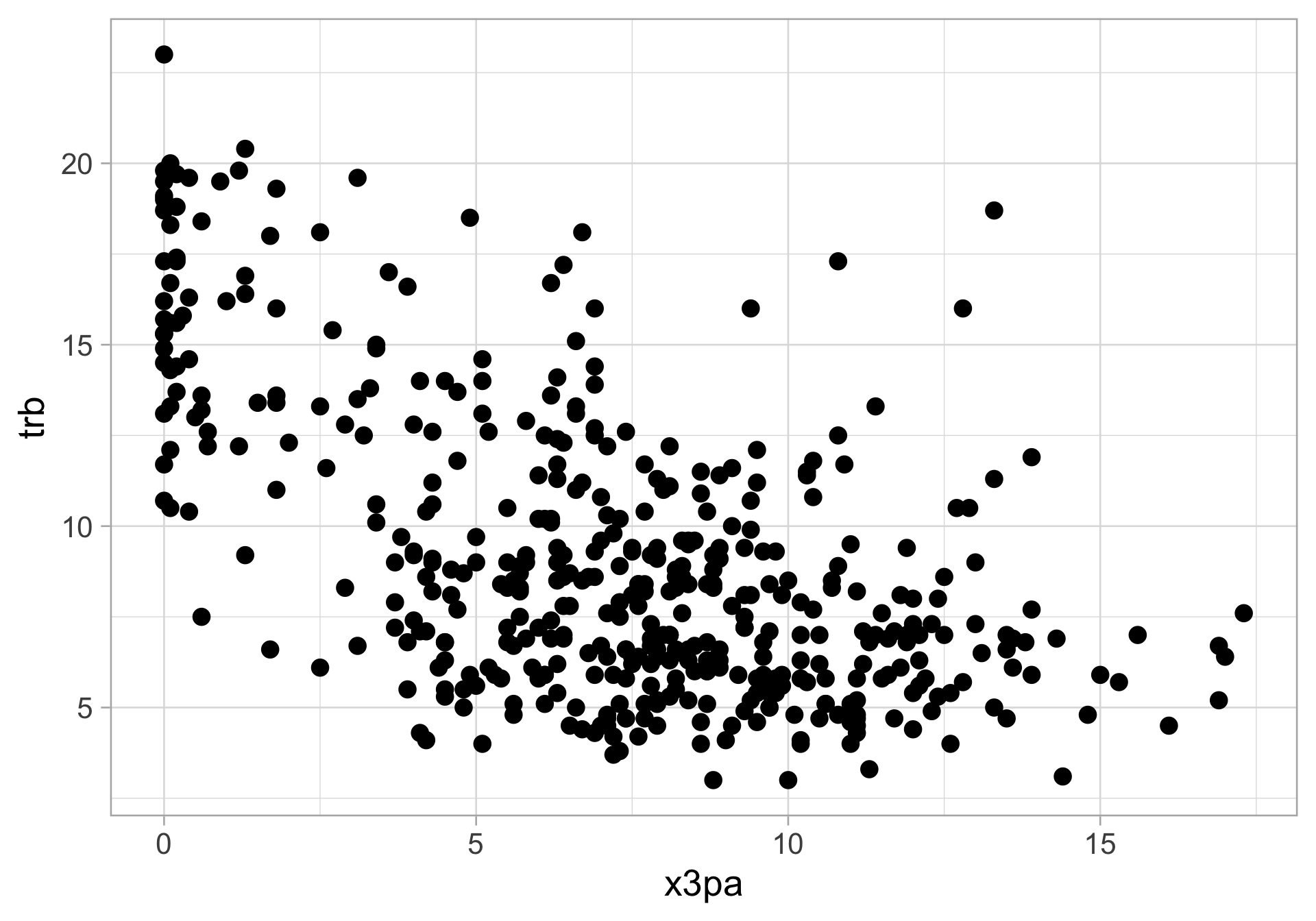
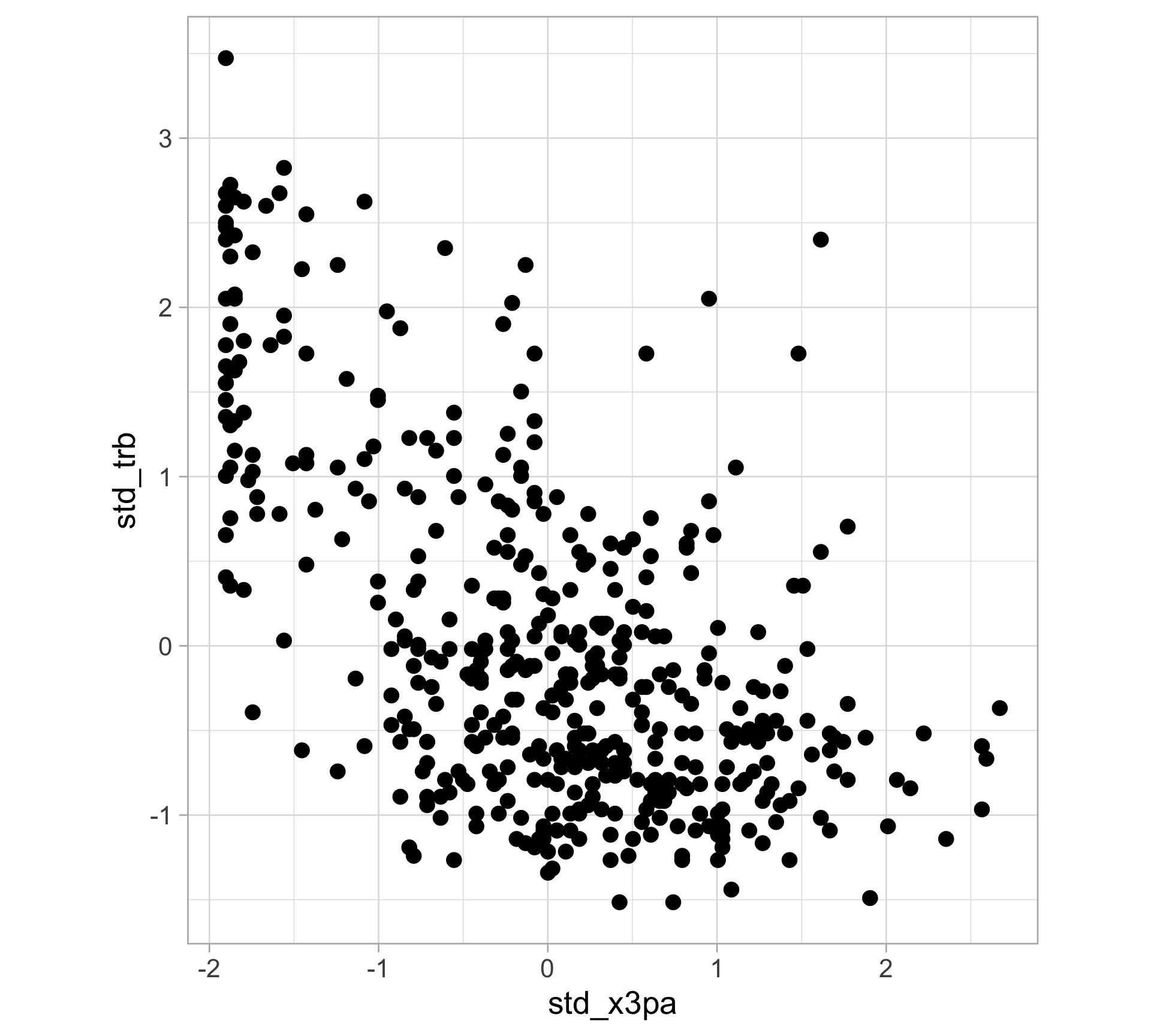
$ x3pa         <dbl> 10.6, 10.0, 6.7, 5.7, 11.1, 8.3, 9.3, 17.0, 0.1, 4.8, 9.5…
$ x3p_percent  <dbl> 0.427, 0.327, 0.267, 0.436, 0.398, 0.431, 0.383, 0.194, 0…
$ x2p          <dbl> 0.8, 4.7, 4.3, 6.3, 2.8, 4.6, 6.2, 2.6, 7.4, 5.5, 2.4, 1.…
$ x2pa         <dbl> 1.8, 8.8, 9.2, 10.8, 5.3, 7.9, 10.7, 5.7, 10.4, 10.0, 4.4…
$ x2p_percent  <dbl> 0.443, 0.528, 0.472, 0.582, 0.517, 0.587, 0.578, 0.458, 0…
$ e_fg_percent <dbl> 0.612, 0.508, 0.441, 0.607, 0.571, 0.617, 0.577, 0.333, 0…
$ ft           <dbl> 0.6, 4.3, 2.4, 4.8, 2.1, 3.1, 2.0, 0.2, 3.6, 2.3, 1.0, 2.…
$ fta          <dbl> 0.8, 6.2, 2.8, 5.9, 2.5, 3.4, 2.4, 0.5, 5.4, 2.8, 1.1, 2.…
$ ft_percent   <dbl> 0.815, 0.683, 0.865, 0.810, 0.829, 0.913, 0.831, 0.500, 0…
$ orb          <dbl> 0.5, 2.0, 0.6, 2.7, 0.8, 1.6, 2.2, 1.7, 5.0, 1.4, 2.4, 0.…
$ drb          <dbl> 4.5, 6.5, 3.8, 5.5, 4.0, 6.0, 5.9, 4.7, 8.3, 4.0, 8.8, 6.…
$ trb          <dbl> 5.1, 8.5, 4.4, 8.2, 4.8, 7.6, 8.1, 6.4, 13.3, 5.5, 11.2, …
$ ast          <dbl> 3.1, 3.1, 5.7, 5.5, 5.1, 2.3, 3.7, 2.8, 1.5, 5.1, 3.9, 3.…
$ stl          <dbl> 1.1, 1.3, 0.9, 0.8, 1.2, 1.5, 1.7, 1.9, 1.4, 2.0, 1.1, 1.…
$ blk          <dbl> 0.2, 0.6, 0.2, 0.5, 0.7, 0.7, 0.5, 0.7, 3.8, 0.3, 1.5, 0.…
$ tov          <dbl> 1.2, 1.5, 2.6, 2.4, 2.3, 1.6, 1.9, 0.9, 3.3, 2.3, 1.4, 1.…
$ pf           <dbl> 4.6, 4.4, 3.7, 2.7, 3.9, 4.9, 2.8, 3.5, 6.8, 5.5, 2.4, 2.…
$ pts          <dbl> 15.8, 23.4, 16.4, 24.9, 20.9, 23.2, 25.2, 15.4, 18.4, 18.…
$ o_rtg        <dbl> 119, 113, 98, 129, 121, 124, 119, 80, 123, 117, 121, 117,…
$ d_rtg        <dbl> 117, 116, 123, 120, 114, 116, 110, 110, 115, 111, 111, 11…
$ awards       <lgl> NA, NA, NA, NA, NA, NA, NA, NA, NA, NA, NA, NA, NA, NA, N…

General setup

Given a dataset with \(p\) variables (columns) and \(n\) observations (rows) \(x_1,\dots,x_n\)
Compute the distance/dissimilarity between observations
e.g. Euclidean distance between observations \(i\) and \(j\)

\[d_{ij} = \sqrt{(x_{i1}-x_{j1})^2 + \cdots + (x_{ip}-x_{jp})^2}\]

What are the distances between these counties using x3pa (3-point attempts) and trb (total rebounds)?

nba_players |> 
  ggplot(aes(x = x3pa, y = trb)) +
  geom_point(size = 4)

Remember to standardize!

nba_players <- nba_players |> 
  mutate(
    std_x3pa = as.numeric(scale(x3pa)),
    std_trb = as.numeric(scale(trb))
  )

nba_players |> 
  ggplot(aes(x = std_x3pa, y = std_trb)) +
  geom_point(size = 4) +
  coord_fixed()

Compute the distance matrix using `dist()`

Compute pairwise Euclidean distance

players_dist <- nba_players |> 
  select(std_x3pa, std_trb) |> 
  dist()

Returns an object of dist class… but not a matrix
Convert to a matrix, then set the row and column names:

players_dist_matrix <- as.matrix(players_dist)
rownames(players_dist_matrix) <- nba_players$player
colnames(players_dist_matrix) <- nba_players$player
players_dist_matrix[1:4, 1:4]

             A.J. Green A.J. Lawson AJ Johnson Aaron Gordon
A.J. Green    0.0000000   0.8626792  1.0457677    1.5086463
A.J. Lawson   0.8626792   0.0000000  1.3441734    1.1393048
AJ Johnson    1.0457677   1.3441734  0.0000000    0.9839163
Aaron Gordon  1.5086463   1.1393048  0.9839163    0.0000000

Hierarchical clustering

Hierarchical clustering in simple terms

Key idea: Builds a hierarchy in a agglomerative/bottom-up fashion
Algorithm (informal version)
- Start with each point in its own cluster
- Identify the closest two clusters and merge them
- Repeat
- Ends when all points are in a single cluster

Toy example

Toy example

Hierarchical clustering

Start with all observations in their own cluster

Step 1: Compute the pairwise dissimilarities between each cluster
- e.g., distance matrix on previous slides (using Euclidean distance)
- In practice, we can also try out different types of distance

Step 2: Identify the pair of clusters that are least dissimilar

Step 3: Fuse these two clusters into a new cluster

Repeat Steps 1 to 3 until all observations are in the same cluster

“Bottom-up”, agglomerative clustering that forms a tree/hierarchy of merging

No mention of any randomness. And no mention of the number of clusters \(k\).

Dissimilarity between clusters

We know how to compute distance/dissimilarity between two observations

But what about distance/dissimilarity between a cluster and an observation, or between two clusters?

We need to choose a linkage function. Clusters are built up by linking them together

Linkages

Linkage: function \(d(C_1, C_2)\) that takes two groups (clusters) \(C_1\) and \(C_2\) and returns a dissimilarity score between them

First, compute all pairwise dissimilarities between the observations in the two clusters (i.e., compute the distance matrix between observations)

Agglomerative clustering, given the linkage:
- Start with all points in their own cluster
- Until there is only one cluster, repeatedly: merge the two clusters \(C_1\), \(C_2\) such that \(d(C_1, C_2)\) is the smallest

There are different types of linkage: complete, single, average,…

Complete linkage

In complete linkage, we use the largest dissimilarity between two points of different clusters (maximal inter-cluster dissimilarity) \[d_\text{complete}(C_1, C_2) = \underset{i \in C_1, j \in C_2}{\text{max}} d_{ij}\]

Below, the complete linkage score \(d_\text{complete}(C_1, C_2)\) is the distance of the furthest pair

Single linkage

In single linkage, we use the smallest dissimilarity between two points of different clusters (minimal inter-cluster dissimilarity) \[d_\text{single}(C_1, C_2) = \underset{i \in C_1, j \in C_2}{\text{min}} d_{ij}\]

Below, the single linkage score \(d_\text{single}(C_1, C_2)\) is the distance of the closest pair

Average linkage

In average linkage, we use the average dissimilarity over all points of different clusters (mean inter-cluster dissimilarity) \[d_\text{average}(C_1, C_2) = \frac{1}{|C_1||C_2|} \sum_{i \in C_1, j \in C_2} d_{ij}\]

In short, the average linkage score \(d_\text{average}(C_1, C_2)\) is the average distance across all pairs (of different clusters)

Complete linkage example

Use hclust() with a dist() objsect
Use complete linkage by default

nba_complete <- players_dist |> 
  hclust(method = "complete")

Use cutree() to return cluster labels
Returns compact clusters (similar to \(k\)-means)

nba_players |> 
  mutate(
    cluster = as.factor(cutree(nba_complete, k = 3))
  ) |>
  ggplot(aes(x = std_x3pa, y = std_trb,
             color = cluster)) +
  geom_point(size = 4) + 
  ggthemes::scale_color_colorblind() +
  theme(legend.position = "bottom")

What are we cutting? Dendrograms

Use the ggdendro package (instead of plot())

library(ggdendro)
nba_complete |> 
  ggdendrogram(labels = FALSE, 
               leaf_labels = FALSE,
               theme_dendro = FALSE) +  
  labs(y = "Dissimilarity between clusters") +
  theme(axis.text.x = element_blank(), 
        axis.title.x = element_blank(),
        panel.grid = element_blank())

Each leaf is one observation
Height of branch indicates dissimilarity between clusters
- (After first step) Horizontal position along x-axis means nothing

Some notes on dendrograms

Dendrograms are often misinterpreted

Conclusions about the distance/dissimilarity between two observations should not be implied by their relationship on the horizontal axis nor by the vertical connections

Rather, the height of the branch between an observation and the clusters of observations below them indicate the distance between the observation and that cluster it is joined to

Toy example

Consider observations 9 and 2. They appear close on the dendrogram
But their closeness on the dendrogram imply they are approximately the same distance measure from the cluster that they are fused to (observations 5, 7, 8)
It by no means implies that observation 9 and 2 are close to one another.

Cut dendrograms to obtain cluster labels

Specify the height to cut with h (instead of k)

For example, cutree(nba_complete, h = 4)

Single linkage example

Change the method argument to single

Results in a chaining effect

Average linkage example

Change the method argument to average

Closer to complete but varies in compactness

Shortcomings of different types of linkage

Single linkage suffers from chaining
- In order to merge two groups, only need one pair of points to be close, irrespective of all others
- Therefore clusters can be too spread out, and not compact enough

Complete linkage avoids chaining, but suffers from crowding
- Because its score is based on the maximum dissimilarity between pairs, a point can be closer to points in other clusters than to points in its own cluster
- Clusters are compact, but not far enough apart

Average linkage tries to strike a balance
- It uses average pairwise dissimilarity, so clusters tend to be relatively compact and relatively far apart
- But it is not clear what properties the resulting clusters have when we cut an average linkage tree at given height.
- Single and complete linkage trees each has simple interpretations

Complete linkage interpretation

Cutting the tree at \(h = 5\) gives the clustering assignments marked by colors
Cut interpretation: for each point \(x_i\), every other point \(x_j\) in its cluster satisfies \(d_{ij} \le 5\)

Single linkage interpretation

Cutting the tree at \(h = 0.9\) gives the clustering assignments marked by colors
Cut interpretation: for each point \(x_i\), there is another point \(x_j\) in its cluster satisfies \(d_{ij} \le 0.9\)

Post-clustering analysis

For context, how does position relate clustering results?
Two-way table to compare the clustering assignments with player positions
(What’s the way to visually compare these two variables?)

table("Cluster" = cutree(nba_complete, k = 3), "Position" = nba_players$pos)

       Position
Cluster   C  PF  PG  SF  SG
      1  15  40  69  51 100
      2   4  25  15  22  19
      3  70  20   1   5   1

Takeaway: positions tend to fall within particular clusters

Include more variables

It’s easy to include more variables - just change the distance matrix

nba_players_features <- nba_players |> 
  select(x3pa, x2pa, fta, trb, ast, stl, blk, tov)
  
player_dist_mult_features <- nba_players_features |> 
  dist(method = "euclidean") # can try out other methods

Then perform hierarchical clustering as before

nba_players_hc_complete <- player_dist_mult_features |> 
  hclust(method = "complete") # can try out other methods

Visualize with dendrogram

nba_players_hc_complete |> 
  ggdendrogram(labels = FALSE, 
               leaf_labels = FALSE,
               theme_dendro = FALSE) +
  labs(y = "Dissimilarity between clusters") +
  theme(axis.text.x = element_blank(), 
        axis.title.x = element_blank(),
        panel.grid = element_blank())

Visualizing clustering results with PCA

Similar to \(k\)-means, if there are more than two dimensions (variables), we can perform PCA
Then plot the observations onto the first two principal components

library(factoextra)
fviz_cluster(
  list(data = nba_players_features,
       cluster = cutree(nba_players_hc_complete, k = 3)),
  geom = "point",
  ellipse = FALSE
) +
  ggthemes::scale_color_colorblind() +
  theme_light()

Choosing number of clusters

Just like \(k\)-means, there are heuristics for choosing the number of clusters for hierarchical clustering
Options: elbow method, silhouette, gap statistic (but again, use these with caution)

nba_players_features |> 
  fviz_nbclust(FUN = hcut, method = "wss")

# silhouette
# nba_players_features |> 
#   fviz_nbclust(FUN = hcut, method = "silhouette")

# gap statistic
# library(cluster)
# nba_hc_gap_stat <- nba_players_features |> 
#   clusGap(FUN = hcut, nstart = 30, K.max = 10, B = 50)
# nba_hc_gap_stat |> 
#   fviz_gap_stat()

Practical issues

What dissimilarity measure should be used?
What type of linkage should be used?
How many clusters to choose?
Which features should we use to drive the clustering?
- Categorical variables?
Hard clustering vs. soft clustering
- Hard clustering (\(k\)-means, hierarchical): assigns each observation to exactly one cluster
- Soft (fuzzy) clustering: assigns each observation a probability of belonging to a cluster

Appendix

Code to build dataset

library(tidyverse)
library(rvest)
nba_url <- "https://www.basketball-reference.com/leagues/NBA_2025_per_poss.html"
nba_players <- nba_url |> 
  read_html() |> 
  html_element(css = "#per_poss") |> 
  html_table() |> 
  janitor::clean_names() |> 
  group_by(player) |> 
  slice_max(g) |> 
  ungroup() |> 
  filter(mp >= 200) # keep players with at least 200 minutes played

Unsupervised learning: hierarchical clustering

Background

The big picture

Data: NBA player statistics per 100 possessions (2024-25 regular season)

General setup

Remember to standardize!

Compute the distance matrix using dist()

Hierarchical clustering

Hierarchical clustering in simple terms

Toy example

Hierarchical clustering

Dissimilarity between clusters

Linkages

Complete linkage

Single linkage

Average linkage

Complete linkage example

What are we cutting? Dendrograms

Some notes on dendrograms

Toy example

Cut dendrograms to obtain cluster labels

Single linkage example

Average linkage example

Shortcomings of different types of linkage

Complete linkage interpretation

Single linkage interpretation

More linkage functions

Post-clustering analysis

Include more variables

Visualizing clustering results with PCA

Choosing number of clusters

Practical issues

Appendix

Code to build dataset

Compute the distance matrix using `dist()`