Data visualization: density estimation

SURE 2025

Department of Statistics & Data Science
Carnegie Mellon University

Background

Data: Caitlin Clark’s shots

Shot attempts by the Caitlin Clark in the 2024 WNBA season using wehoop

library(tidyverse)
theme_set(theme_light())
clark_shots <- read_csv("https://raw.githubusercontent.com/36-SURE/2025/main/data/clark_shots.csv")
glimpse(clark_shots)

Rows: 658
Columns: 6
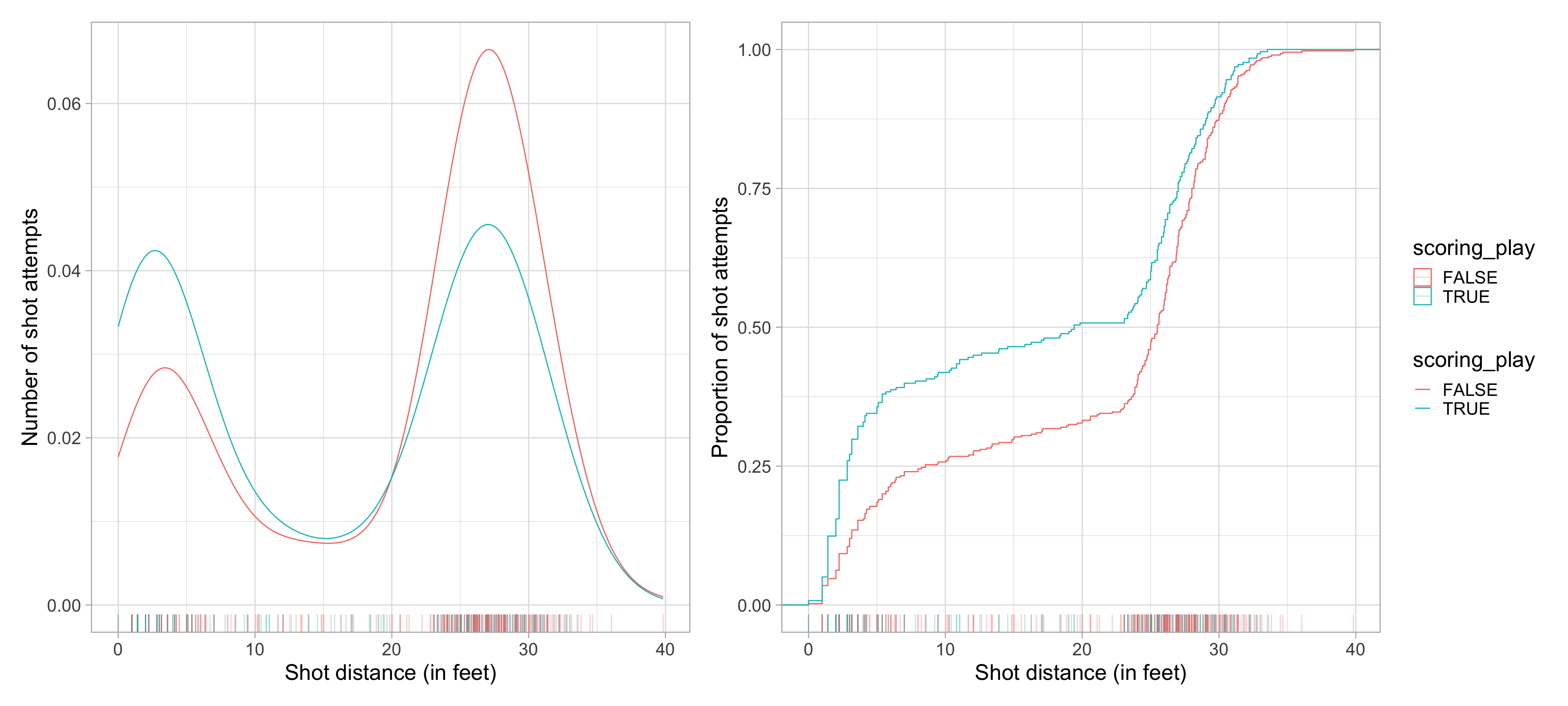
$ scoring_play  <lgl> TRUE, FALSE, FALSE, TRUE, FALSE, FALSE, TRUE, FALSE, TRU…
$ score_value   <dbl> 3, 0, 0, 3, 0, 0, 2, 0, 2, 0, 0, 2, 2, 0, 2, 0, 2, 0, 0,…
$ shot_x        <dbl> -17, -1, -14, -17, -18, -1, 5, 6, 1, -16, -19, 0, 2, -7,…
$ shot_y        <dbl> 22, 33, 16, 19, 20, 0, 6, 30, 1, 21, 13, 4, 1, 32, 1, 14…
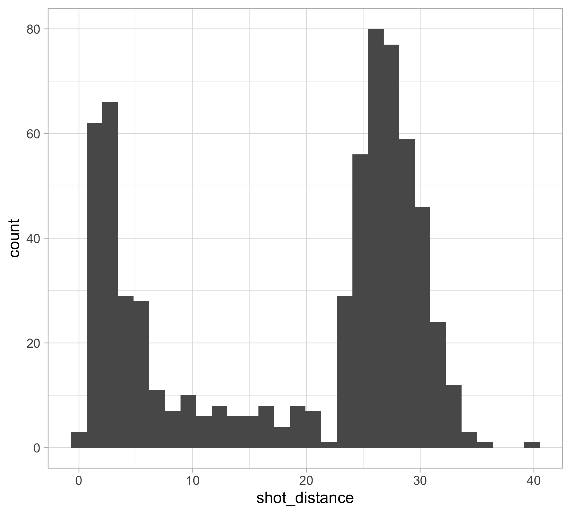
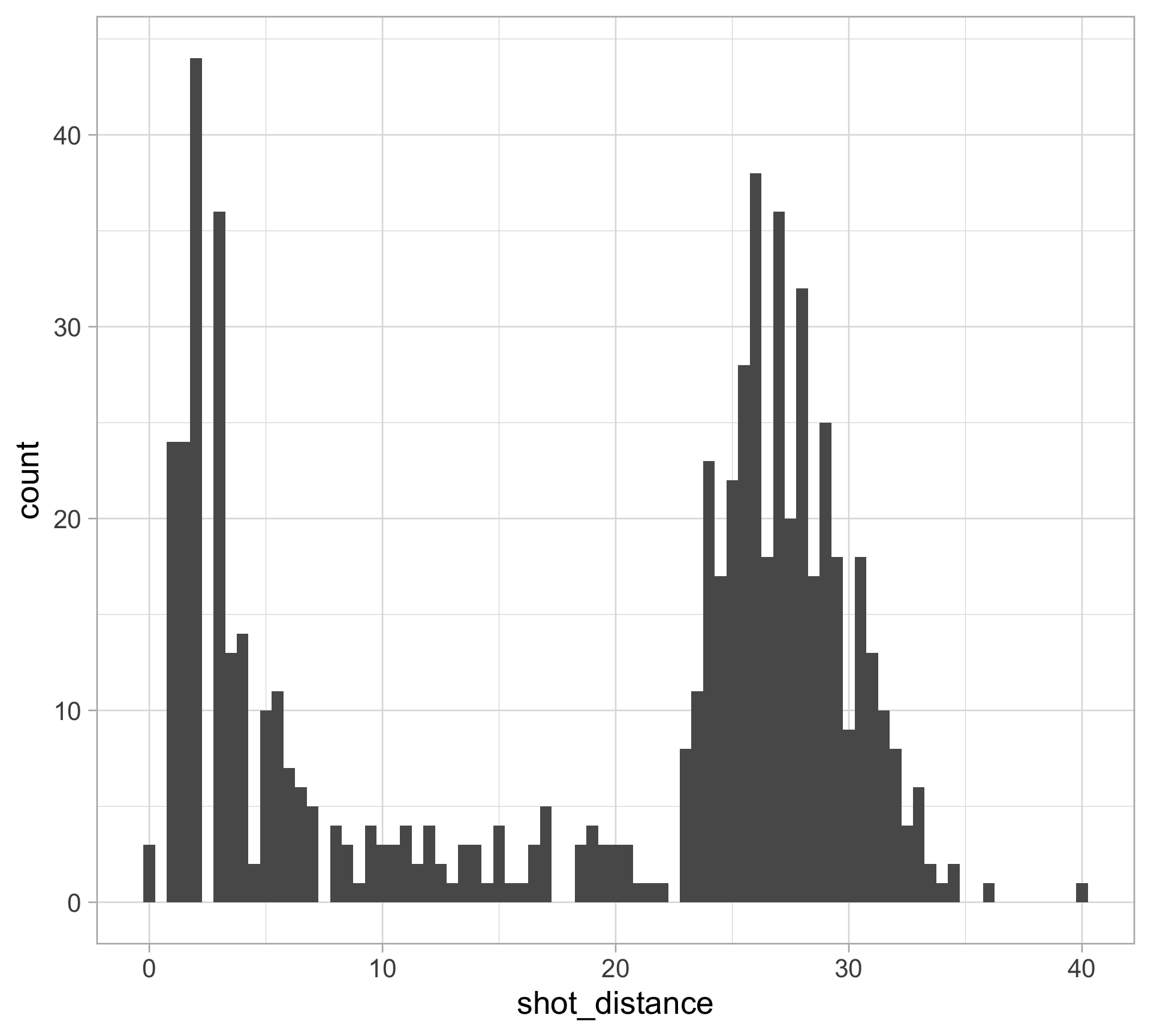
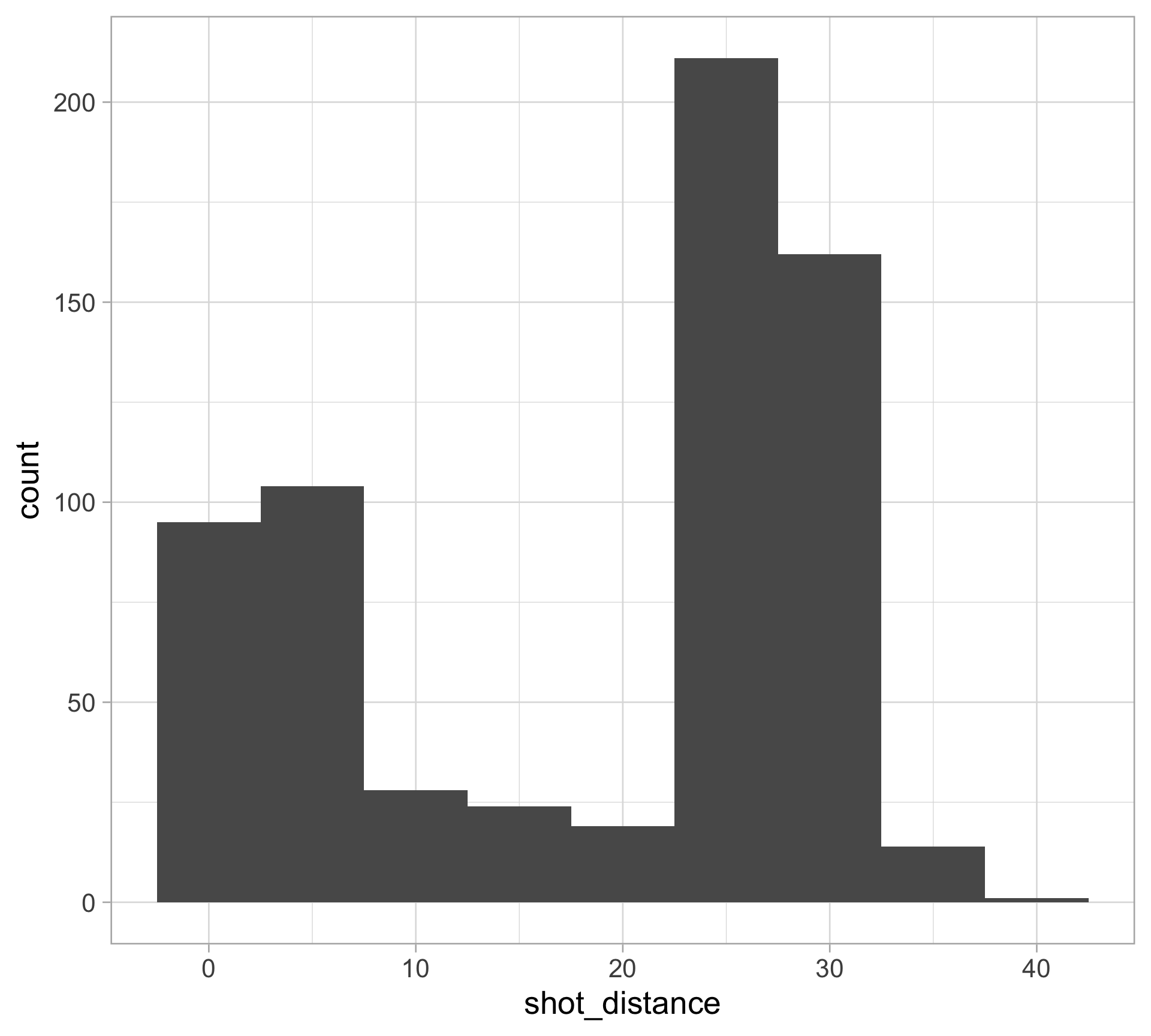
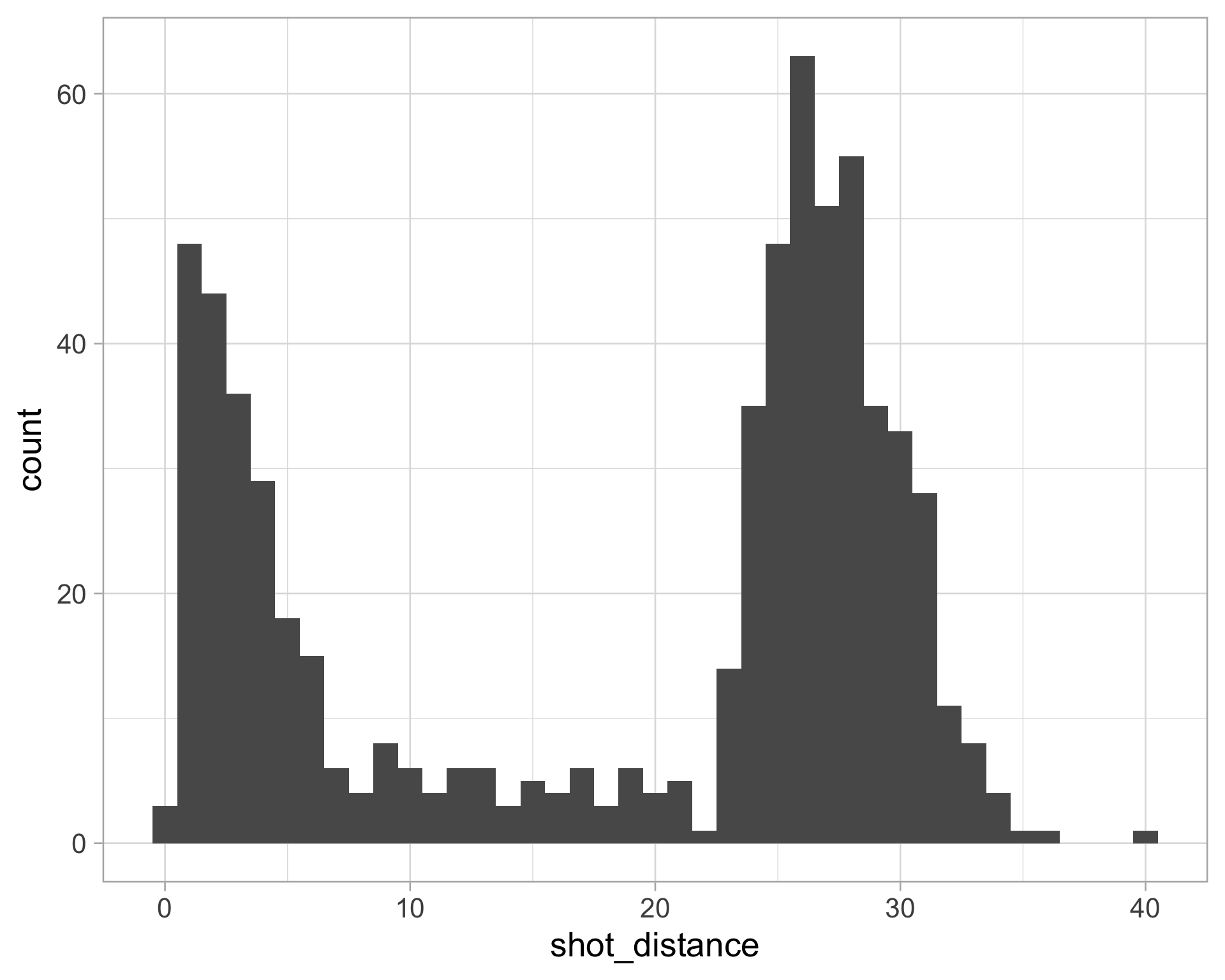
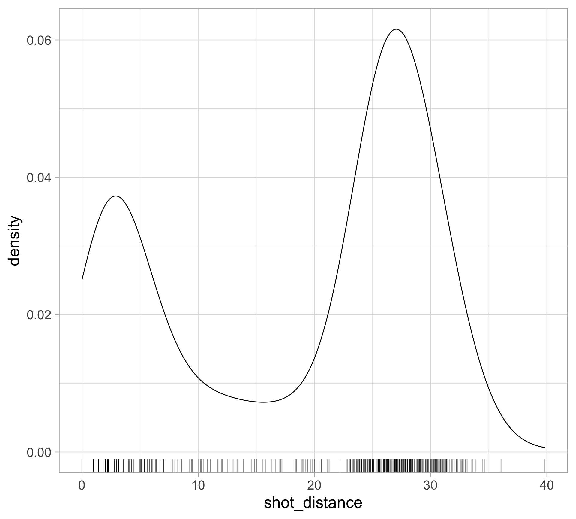
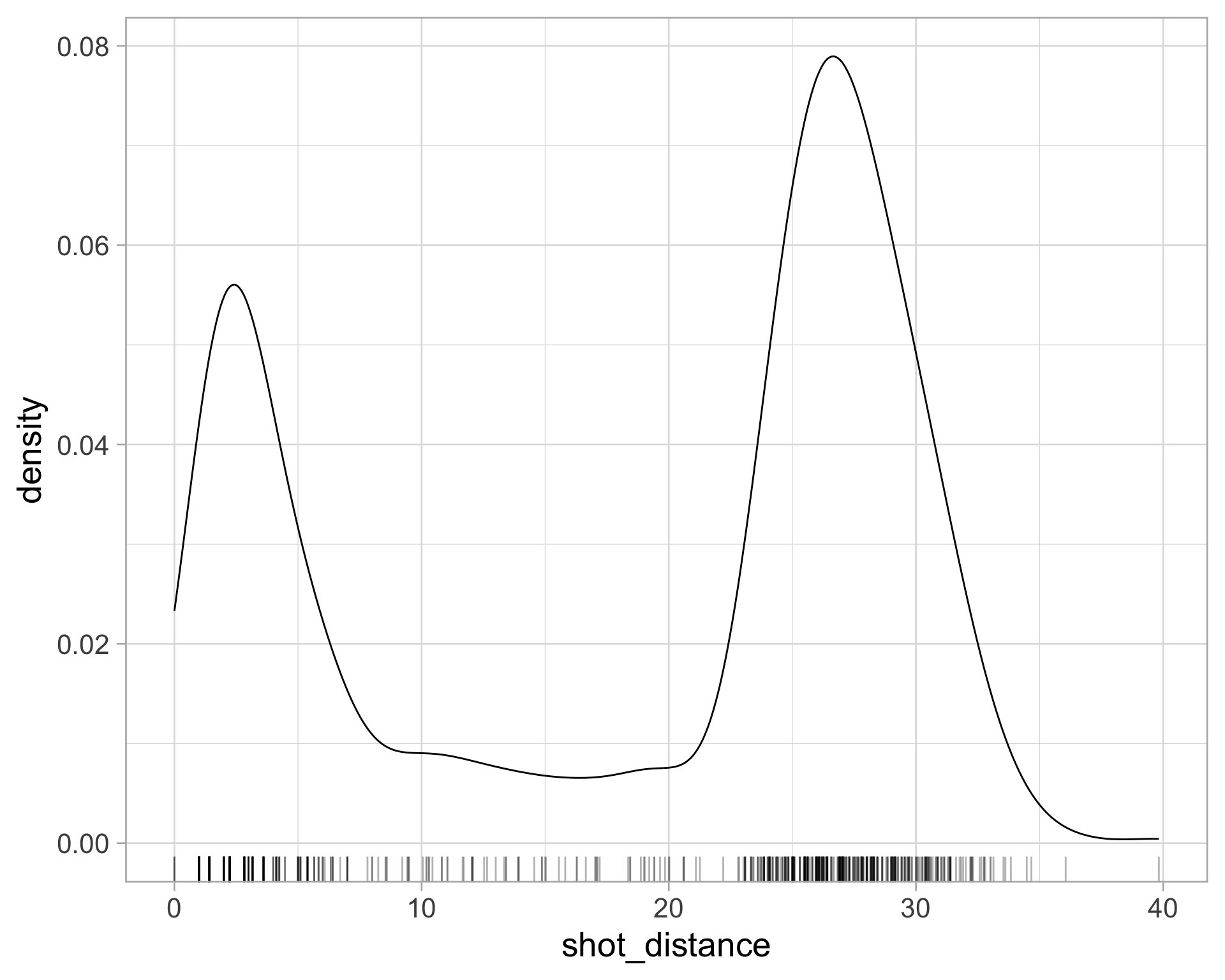
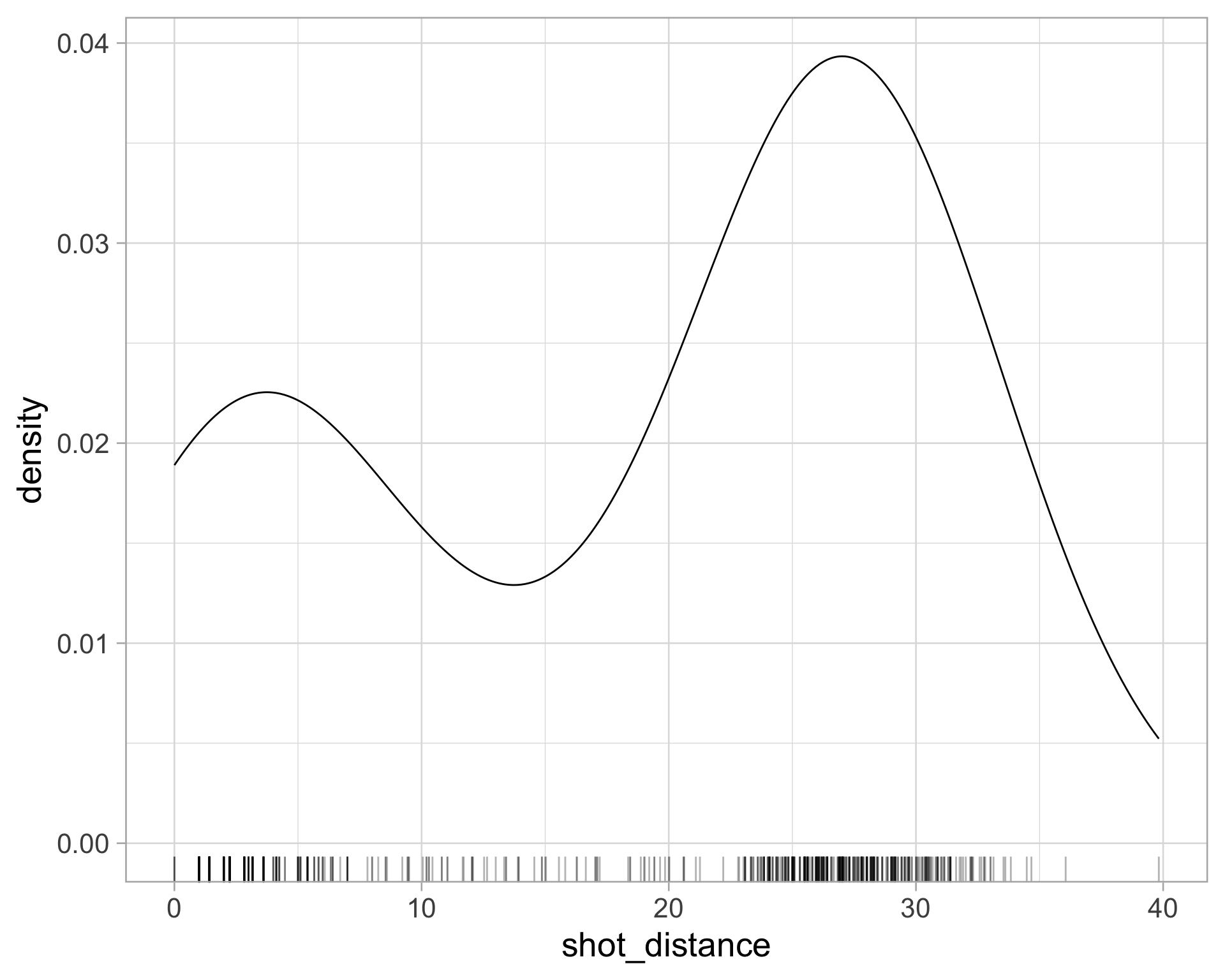
$ shot_distance <dbl> 27.802878, 33.015148, 21.260292, 25.495098, 26.907248, 1…
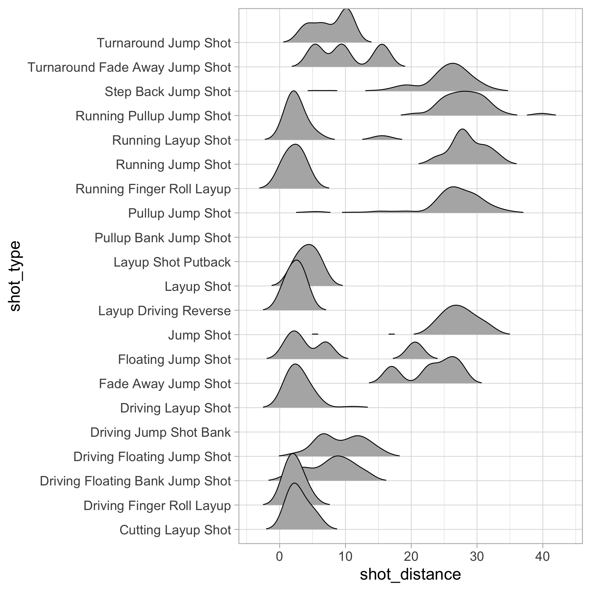
$ shot_type     <chr> "Running Pullup Jump Shot", "Pullup Jump Shot", "Step Ba…

• Each row is a shot attempt by Caitlin Clark in the 2024 WNBA season

• Categorical/qualitative variables: scoring_play, shot_type

• Continuous/quantitative variables: shot_x, shot_y, shot_distance, score_value

Revisiting histograms

Revisiting histograms

clark_shots |>
  ggplot(aes(x = shot_distance)) +
  geom_histogram()

• Split observed data into bins

• Count number of observations in each bin

Need to choose the number of bins, adjust with:

• bins: number of bins (default is 30)

• binwidth: width of bins (overrides bins), various rules of thumb

• breaks: vector of bin boundaries (overrides both bins and binwidth)

Adjusting the binwidth

Small binwidth \(\rightarrow\) undersmooth/spiky

clark_shots |>
  ggplot(aes(x = shot_distance)) +
  geom_histogram(binwidth = 0.5)

Large binwidth \(\rightarrow\) oversmooth/flat

clark_shots |>
  ggplot(aes(x = shot_distance)) +
  geom_histogram(binwidth = 5)

Adjusting the binwidth

• A binwidth that is too narrow shows too much detail

  • too many bins: low bias, high variance

• A binwidth that is too wide hides detail

  • too few bins: high bias, low variance

• Always pick a value that is “just right” (The Goldilocks principle, the “baby bear”)

Try several values, the ggplot2 default is NOT guaranteed to be an optimal choice

A subtle point about the histogram code…

By default the bins are centered on the integers

• left-closed, right-open intervals
• starting at -0.5 to 0.5, 0.5 to 1.5, …

clark_shots |>
  ggplot(aes(x = shot_distance)) +
  geom_histogram(binwidth = 1)

Specify center of one bin (e.g. 0.5)

• Use closed = "left"

clark_shots |>
  ggplot(aes(x = shot_distance)) +
  geom_histogram(binwidth = 1, center = 0.5, 
                 closed = "left")

How do histograms relate to the PDF & CDF?

• Histograms approximate the PDF with bins, and points are equally likely within a bin

• PDF is the derivative of the cumulative distribution function (CDF)

Density estimation

Kernel density estimation: intuition

• smooth each data point into a small density bumps
• sum all these small bumps together to obtain the final density estimate

Check out this great interactive tutorial

Kernel density estimation (KDE)

Goal: estimate the PDF \(f(x)\) for all possible values (assuming it is smooth)

The kernel density estimator (KDE) is \(\displaystyle \hat{f}(x) = \frac{1}{n} \sum_{i=1}^n \frac{1}{h} K_h(x - x_i)\)

• \(n\): sample size

• \(x\): new point to estimate \(f(x)\) (does NOT have to be in the dataset!)

• \(h\): bandwidth, analogous to histogram binwidth, ensures \(\hat{f}(x)\) integrates to 1

• \(x_i\): \(i\)th observation in the dataset

• \(K_h(x - x_i)\): kernel function, creates weight given distance of \(i\)th observation from new point

  • as \(|x - x_i| \rightarrow \infty\) then \(K_h(x - x_i) \rightarrow 0\)
    (i.e. the further apart the \(i\)th observation is from \(x\), the smaller the weight)

  • as bandwidth \(h\) increases, weights are more evenly spread out

  • \(K_h(x - x_i)\) is large when \(x_i\) is close to \(x\)

Choice of kernel

The Gaussian (normal) kernel is typically used, but there are many other choices

Visualizing KDE

• We make kernel density estimates with geom_density()

clark_shots |>
  ggplot(aes(x = shot_distance)) + 
  geom_density() +
  geom_rug(alpha = 0.3)

• Pros:
  • Displays full shape of distribution
  • Can easily layer
  • Add categorical variable with color
• Cons:
  • Need to pick bandwidth and kernel…

What about the bandwidth?

See ?geom_density for the default bandwidth

Modify the bandwidth using the adjust argument (value to multiply default bandwidth by)

clark_shots |>
  ggplot(aes(x = shot_distance)) + 
  geom_density(adjust = 0.5) +
  geom_rug(alpha = 0.3)

clark_shots |>
  ggplot(aes(x = shot_distance)) + 
  geom_density(adjust = 2) +
  geom_rug(alpha = 0.3)

Notes on density estimation

• In KDE, the bandwidth parameter is analogous to the binwidth in histograms

• If the bandwidth is too small, the density estimate can become overly peaky and the main trends in the data may be obscured

• If the bandwidth is too large, then smaller features in the distribution of the data may disappear

Notes on density estimation

• The choice of the kernel can affect the shape of the density curve.

  • A Gaussian kernel typically gives density estimates that look bell-shaped (ish)

  • A rectangular kernel can generate the appearance of steps in the density curve

  • Kernel choice matters less with more data points

• What about uncertainty?

Density plots are often reliable and informative for large datasets but can be misleading for smaller ones.

Use density curves and ECDFs together

Code interlude: arranging multiple figures

Use the cowplot package to easily arrange your plots (see also patchwork)

library(cowplot)

clark_shot_dens <- clark_shots |>
  ggplot(aes(x = shot_distance)) + 
  geom_density() +
  geom_rug(alpha = 0.3) +
  theme_bw() +
  labs(x = "Shot distance (in feet)",
       y = "Number of shot attempts")

clark_shot_ecdf <- clark_shots |>
  ggplot(aes(x = shot_distance)) + 
  stat_ecdf() +
  geom_rug(alpha = 0.3) +
  theme_bw() +
  labs(x = "Shot distance (in feet)",
       y = "Proportion of shot attempts")

# library(patchwork)
# clark_shot_dens + clark_shot_ecdf
plot_grid(clark_shot_dens, clark_shot_ecdf)

Use density curves and ECDFs together

Another code interlude: collect the legends with patchwork

clark_shot_dens_made <- clark_shots |>
  ggplot(aes(x = shot_distance, 
             color = scoring_play)) + 
  geom_density() +
  geom_rug(alpha = 0.3) +
  labs(x = "Shot distance (in feet)",
       y = "Number of shot attempts")

clark_shot_ecdf_made <- clark_shots |>
  ggplot(aes(x = shot_distance,
             color = scoring_play)) + 
  stat_ecdf() +
  geom_rug(alpha = 0.3) +
  labs(x = "Shot distance (in feet)",
       y = "Proportion of shot attempts")

library(patchwork)
clark_shot_dens_made + clark_shot_ecdf_made + plot_layout(guides = "collect")

Ridgeline plots

• Check out the ggridges package for a variety of customization options

library(ggridges)
clark_shots |>
  ggplot(aes(x = shot_distance, y = shot_type)) + 
  geom_density_ridges(rel_min_height = 0.01) 

• Useful to display conditional distributions across many levels

• Also check out ggdist (becoming Quang’s favorite)

Going from 1D to 2D density estimation

In 1D: estimate density \(f(x)\), assuming that \(f(x)\) is smooth:

\[ \hat{f}(x) = \frac{1}{n} \sum_{i=1}^n \frac{1}{h} K_h(x - x_i) \]

In 2D: estimate joint density \(f(x_1, x_2)\)

\[\hat{f}(x_1, x_2) = \frac{1}{n} \sum_{i=1}^n \frac{1}{h_1h_2} K\left(\frac{x_1 - x_{i1}}{h_1}\right) K\left(\frac{x_2 - x_{i2}}{h_2}\right)\]

In 1D there’s one bandwidth, now we have two bandwidths

• \(h_1\): controls smoothness as \(X_1\) changes, holding \(X_2\) fixed
• \(h_2\): controls smoothness as \(X_2\) changes, holding \(X_1\) fixed

Gaussian kernels are still a popular choice

Display densities for 2D data: contour plots

Best known in topography: outlines (contours) denote levels of elevation

2D density estimation

We can visualize all of the shot locations: (shot_x, shot_y)

clark_shots |>
  ggplot(aes(x = shot_x, y = shot_y)) +
  geom_point(size = 4, alpha = 0.3)

• Adjust transparency with alpha for overlapping points

Create contours of 2D kernel density estimate

• Use geom_density2d() to display contour lines

clark_shots |>
  filter(shot_y < 35) |> # remove outliers
  ggplot(aes(x = shot_x, y = shot_y)) + 
  geom_point(size = 4, alpha = 0.3) + 
  geom_density2d() +
  coord_fixed() +
  theme(legend.position = "bottom")

• Extend KDE for joint density estimates in 2D (see section 14.4.2 for details)

• Inner lines denote “peaks”

• coord_fixed() forced a fixed ratio

Create contours of 2D kernel density estimate

• We make 2D KDE contour plots using geom_density2d()

clark_shots |>
  filter(shot_y < 35) |> 
  ggplot(aes(x = shot_x, y = shot_y)) + 
  geom_point(size = 4, alpha = 0.3) + 
  geom_density2d(adjust = 0.1) +
  coord_fixed() +
  theme(legend.position = "bottom")

• Can use adjust to modify the multivariate bandwidth

Contours are difficult… what about heatmaps?

• Use stat_density_2d() and the after_stat() function to make 2D KDE heatmaps

• May be easier to read than nested lines with color

• Default color scale is awful. Always change it.

clark_shots |>
  filter(shot_y < 35) |> 
  ggplot(aes(x = shot_x, y = shot_y)) + 
  stat_density2d(aes(fill = after_stat(level)),
                 h = 0.6, bins = 60, geom = "polygon") +
  scale_fill_gradient(low = "midnightblue", 
                      high = "gold") +
  coord_fixed() +
  theme(legend.position = "bottom")

Multivariate density estimation can be difficult

Turn off contours and use tiles instead

• Divide the space into a grid and color the grid according to high/low values

clark_shots |>
  filter(shot_y < 35) |> 
  ggplot(aes(x = shot_x, y = shot_y)) + 
  stat_density2d(aes(fill = after_stat(density)),
                 h = 0.6, bins = 60, contour = FALSE,
                 geom = "raster") +
  # scale_fill_gradient(low = "white", high = "red") +
  scale_fill_gradient(low = "midnightblue", 
                      high = "gold") +
  theme(legend.position = "bottom") +
  coord_fixed()

Best alternative? Hexagonal binning

• Use geom_hex() to make hexagonal heatmaps

• Need to have the hexbin package installed

• 2D version of histogram

clark_shots |>
  filter(shot_y < 35) |>
  ggplot(aes(x = shot_x, y = shot_y)) + 
  geom_hex(binwidth = c(1, 1)) +
  scale_fill_gradient(low = "midnightblue", 
                      high = "gold") + 
  theme(legend.position = "bottom") +
  coord_fixed()

• Can specify binwidth in both directions
• Avoids limitations from smoothing

What about shooting efficiency?

• Can compute a function of another variable inside hexagons with stat_summary_hex()

clark_shots |>
  filter(shot_y < 35) |>
  ggplot(aes(x = shot_x, y = shot_y, 
             z = scoring_play, group = -1)) +
  stat_summary_hex(binwidth = c(2, 2), fun = mean, 
                   color = "black") +
  scale_fill_gradient(low = "midnightblue", 
                      high = "gold") + 
  theme(legend.position = "bottom") +
  coord_fixed()

Appendix: Making shot charts and drawing courts with sportyR

library(sportyR)
wnba_court <- geom_basketball("wnba", display_range = "offense", rotation = 270, x_trans = -41.5)
wnba_court +
  geom_hex(data = clark_shots, aes(x = shot_x, y = shot_y), binwidth = c(1, 1)) + 
  scale_fill_gradient(low = "midnightblue", high = "gold")

Appendix: Code to build dataset

# install.packages("wehoop")
library(wehoop)
wnba_pbp <- load_wnba_pbp(2024)
clark_shots <- wnba_pbp |> 
  filter(shooting_play) |> 
  filter(str_detect(text, "Caitlin Clark")) |> 
  filter(!str_detect(text, "Caitlin Clark assists")) |> 
  filter(!str_detect(text, "free throw")) |> 
  mutate(
    shot_x = coordinate_x_raw - 25,
    shot_y = coordinate_y_raw,
    shot_distance = sqrt((abs(shot_x) ^ 2) + shot_y ^ 2), 
    shot_type = type_text,
    scoring_play,
    score_value,
    .keep = "none"
  )