Simulation

SURE 2025

Department of Statistics & Data Science
Carnegie Mellon University

Background

Why simulation?

• We’re in the 21st century!

• Simulations can often be

  • easier than hand calculations

  • made more realistic than hand calculations

• R provides unique access to great (statistical) simulation tools

Sampling from a given vector

• To sample from a given vector, use sample()

# base R built in English alphabet
# letters
sample(letters, size = 5) # sample without replacement, by default

[1] "l" "k" "z" "w" "o"

sample(c(0, 1), size = 7, replace = TRUE) # sample with replacement

[1] 1 1 0 1 1 0 1

# 5 (independent) coin tosses
coin <- c("H", "T")
sample(coin, 5, replace = TRUE)

[1] "T" "T" "H" "T" "T"

sample(1:100, 1) # sample a random integer between 1 and 100

[1] 65

Probability distributions

A distribution is a mathematical function \(f(x \mid \theta)\) where

• \(x\) may take on continuous or discrete values over the domain (i.e. all possible inputs) of \(f(x \mid \theta)\)
• \(\theta\) is a set of parameters governing the shape of the distribution
  • e.g. \(\theta = \{\mu, \sigma ^2 \}\) for a normal (Gaussian) distribution
• the \(\mid\) symbol means that the shape of the distribution is conditional on the values of \(\theta\)

Let \(f\) denote the distribution for its

• probability density function (PDF) if \(x\) is continuous
• probability mass function (PMF) if \(x\) is discrete

Note:

• \(f(x \mid \theta) \geq 0\) for all \(x\)
• \(\displaystyle \sum_x f(x \mid \theta) = 1\) (discrete case) or \(\displaystyle \int_x f(x \mid \theta) = 1\) (continuous case)

Normal distribution

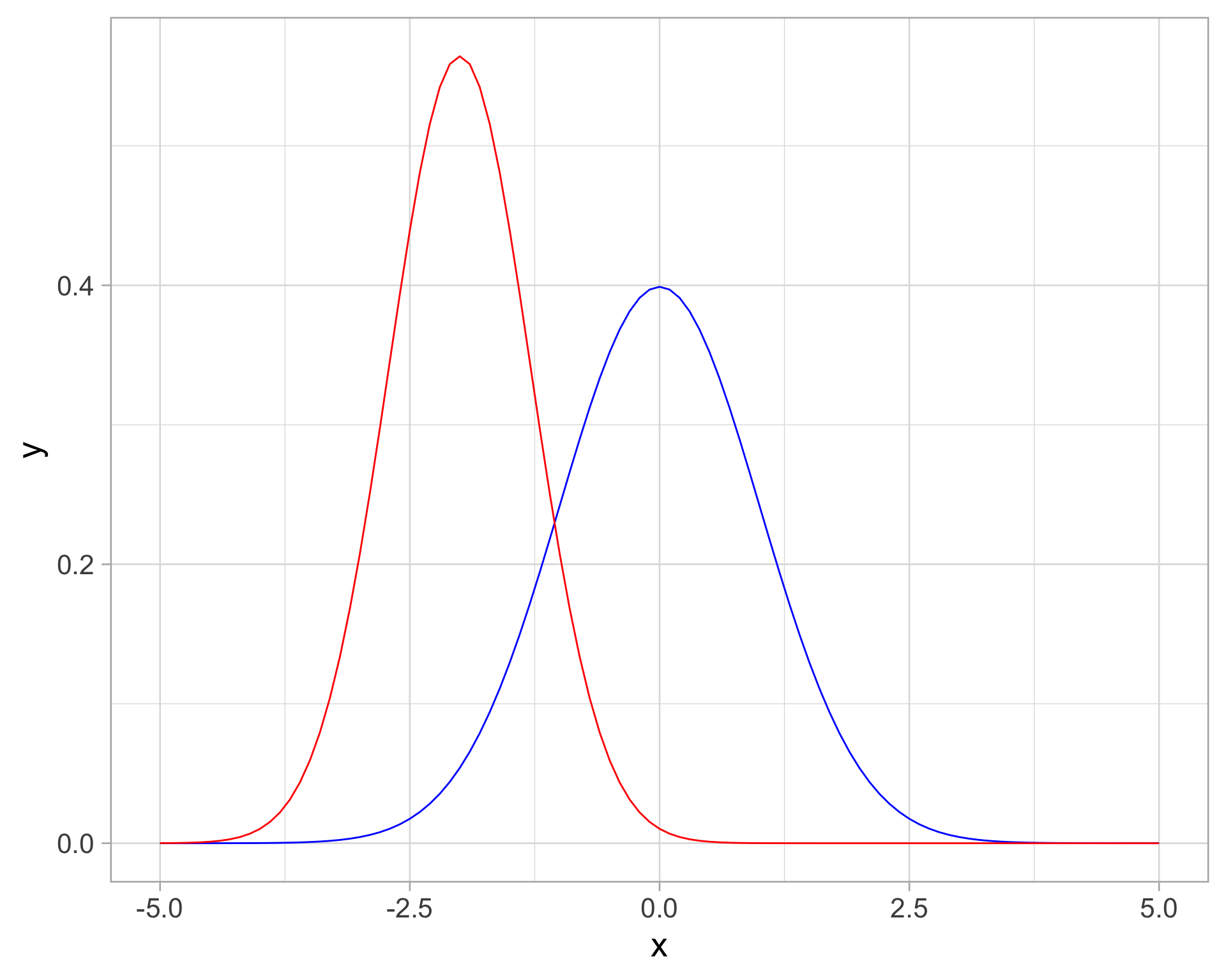
• PDF: \(\displaystyle f(x \mid \mu, \sigma^2)=\frac{1}{\sigma \sqrt{2 \pi}} e^{-\frac{1}{2}\left(\frac{x-\mu}{\sigma}\right)^{2}}\); \(x \in (- \infty, \infty)\)

• We write \(X \sim N(\mu, \sigma^2)\)

• Standard normal distribution: \(N(0, 1)\)

library(tidyverse)
theme_set(theme_light())
tibble(x = c(-5, 5)) |> 
  ggplot(aes(x)) +
  stat_function(fun = dnorm, color = "blue",
                args = list(mean = 0, sd = 1)) +
  stat_function(fun = dnorm, color = "red",
                args = list(mean = -2, sd = sqrt(0.5)))

Binomial distribution

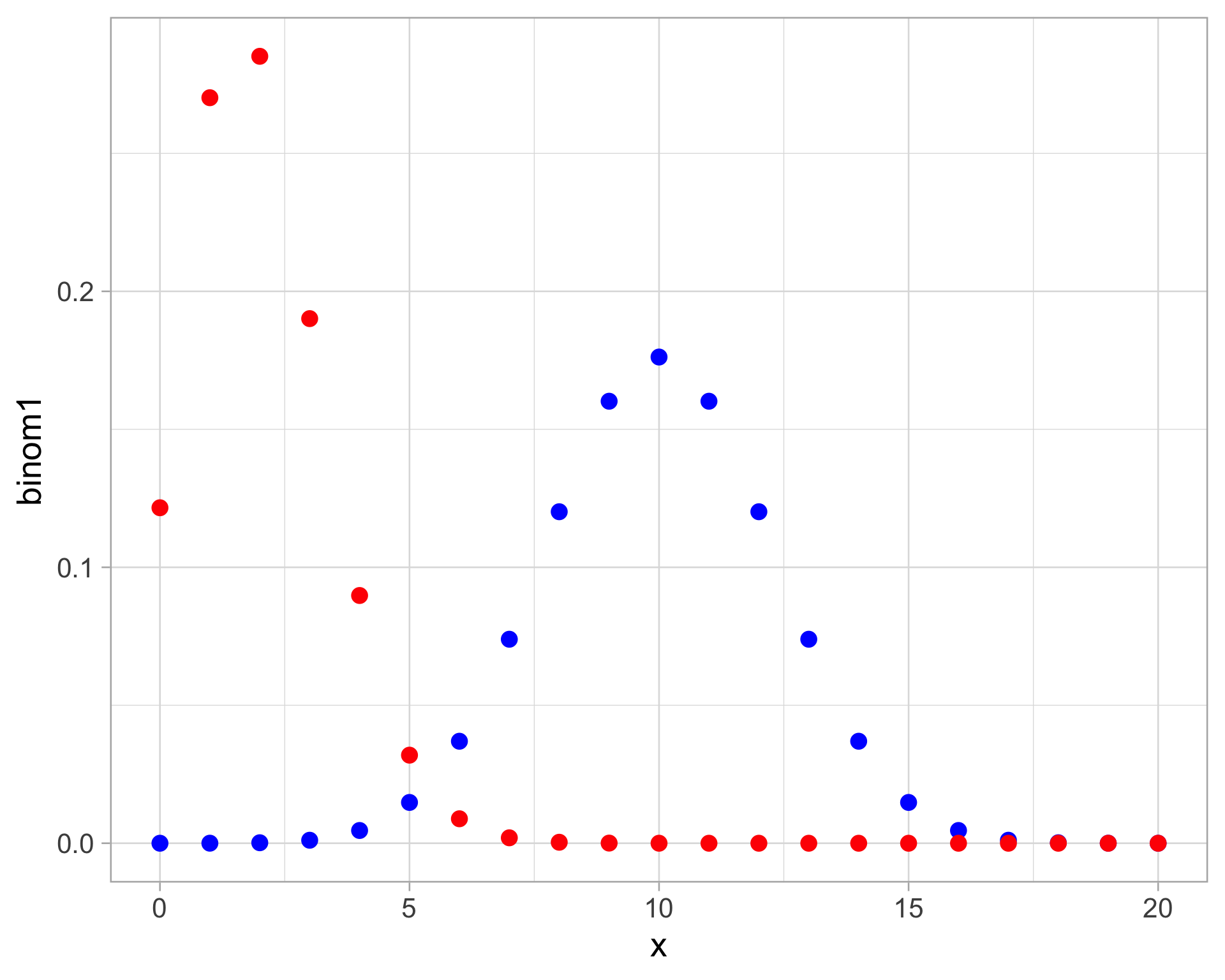
• PMF: \(\displaystyle f(x \mid n, p)= \binom{n}{x} p^{x}(1-p)^{n-x}\); \(x = 0, 1, \dots, n\)

• Model for the probability of \(x\) successes in \(n\) independent trials, each with success probability \(p\)

• We write \(X \sim \text{Binomial}(n,p)\)

tibble(x = 0:20) |>
  mutate(binom1 = dbinom(x, size = 20, prob = 0.5),
         binom2 = dbinom(x, size = 20, prob = 0.1)) |>
  ggplot(aes(x)) + 
  geom_point(aes(y = binom1), color = "blue", size = 4) +
  geom_point(aes(y = binom2), color = "red", size = 4)

Poisson distribution

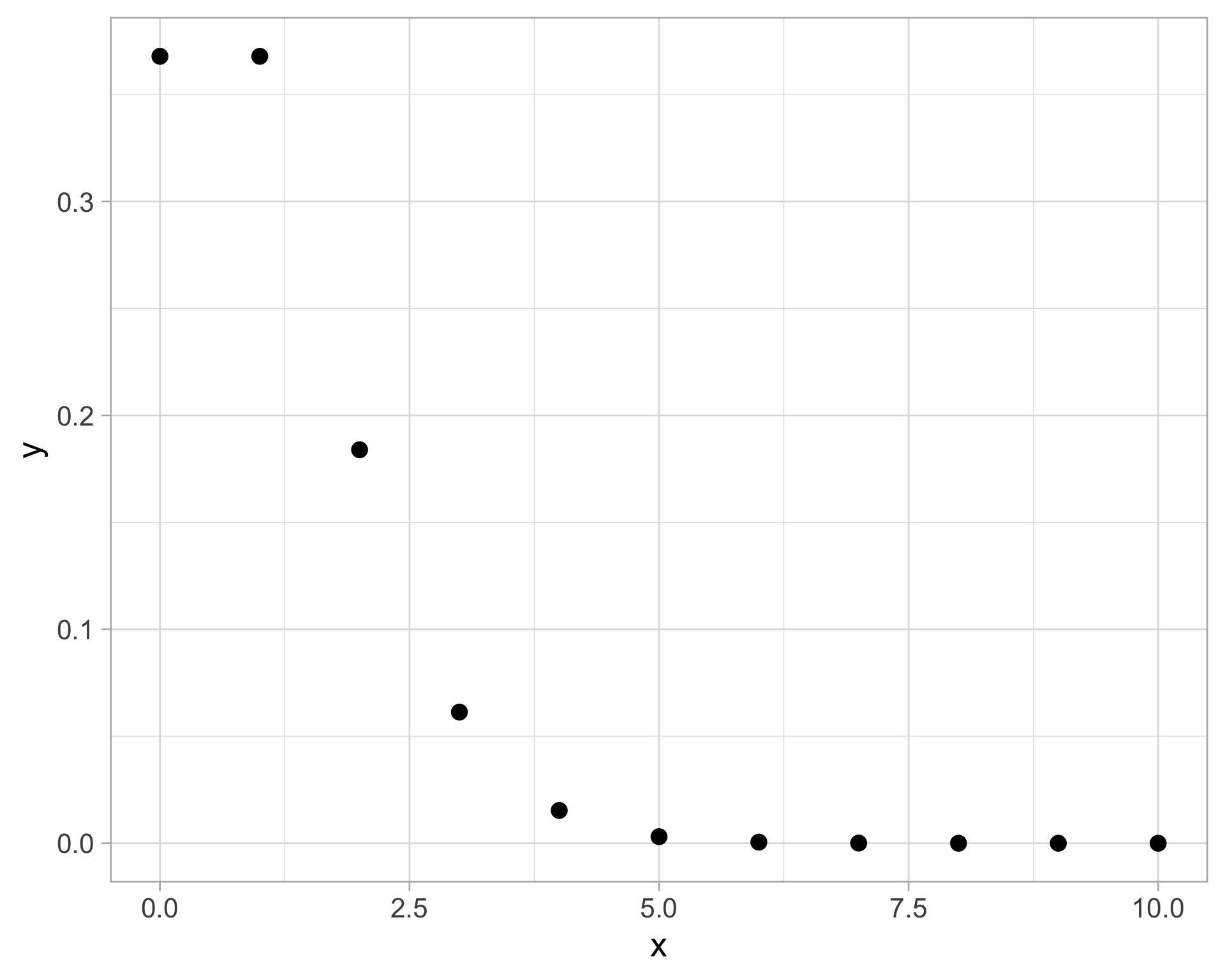
• PMF: \(\displaystyle f(x \mid \lambda)= \frac{ e^{-\lambda} \lambda^x}{x!}\); \(x = 0, 1, 2, \dots\) and \(\lambda > 0\)

• Model for the counts of an event in a fixed period of time, with a rate of occurrence parameter \(\lambda\)

• We write \(X \sim \text{Poisson}(\lambda)\)

tibble(x = 0:10) |> 
  mutate(y = dpois(x, 1)) |> 
  ggplot(aes(x, y)) +
  geom_point(size = 4)

Random number generation

Example: Sampling from a normal distribution

• rnorm(): generate normal random variables

• pnorm(): normal cumulative distribution function

• dnorm(): normal density function

• qnorm(): normal quantile function

Note: Replace “norm” with the name of another distribution, all the same functions apply.

• E.g., “t”, “exp”, “gamma”, “chisq”, “binom”, “pois”, “unif”, etc.

See this manual for more details

Random number generation

# these are the defaults for mean and sd
z <- rnorm(1000, mean = 0, sd = 1)
# check: the sample mean is approximately 0
mean(z) 

[1] -0.04081031

# check: the sample sd is approximately 1
sd(z)

[1] 0.9578959

Revisiting ECDF

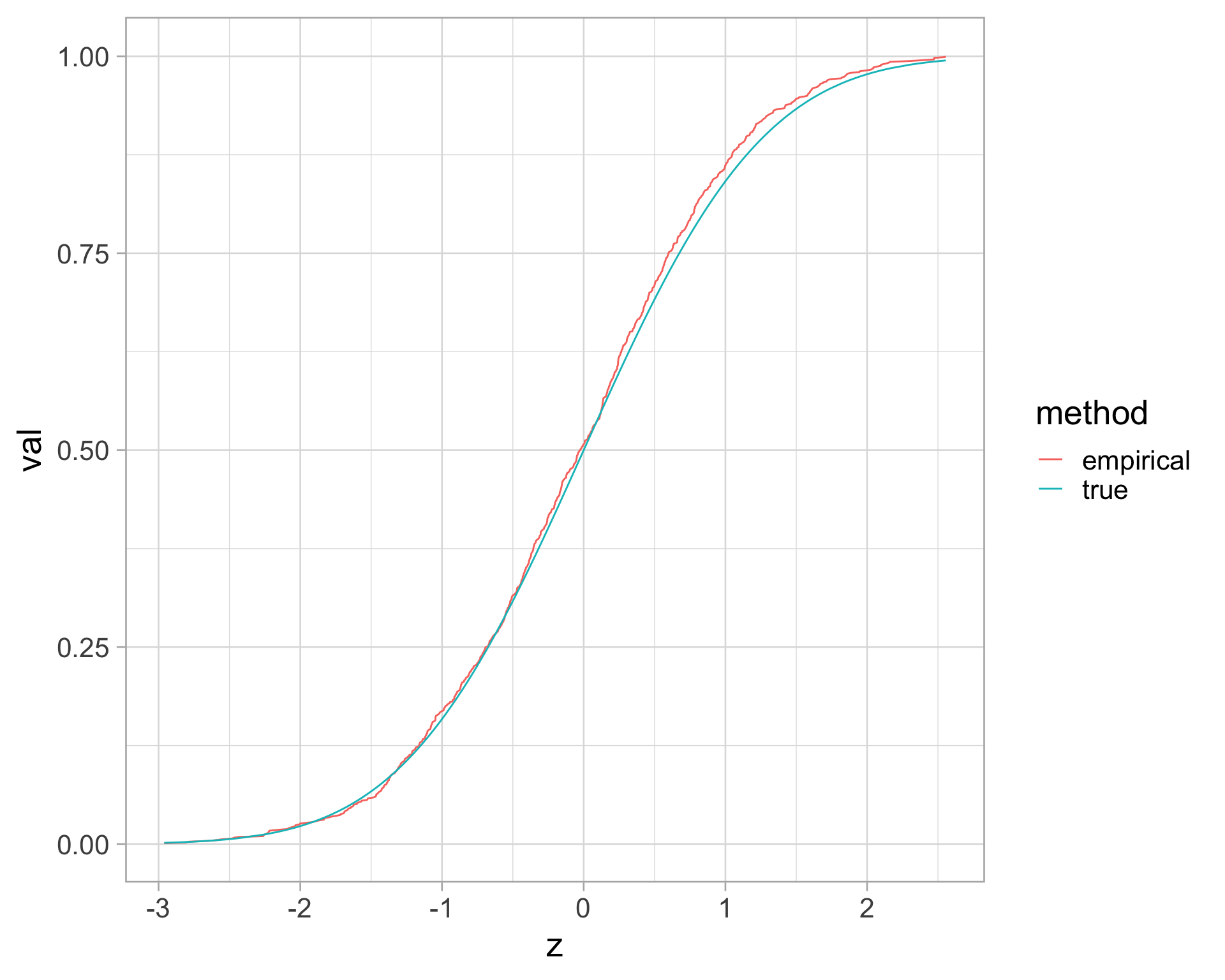
Recall that we can use the ECDF to estimate the true cumulative distribution function

z_ecdf <- ecdf(z)
z_ecdf(0) # should get close to 1/2

[1] 0.507

class(z_ecdf)

[1] "ecdf"     "stepfun"  "function"

normal_tbl <- tibble(z = sort(z)) |> 
  mutate(empirical = z_ecdf(z),
         true = pnorm(z))
normal_tbl

# A tibble: 1,000 × 3
       z empirical    true
   <dbl>     <dbl>   <dbl>
 1 -2.96     0.001 0.00154
 2 -2.81     0.002 0.00248
 3 -2.78     0.003 0.00269
 4 -2.65     0.004 0.00405
 5 -2.59     0.005 0.00486
 6 -2.56     0.006 0.00529
 7 -2.48     0.007 0.00656
 8 -2.47     0.008 0.00679
 9 -2.44     0.009 0.00744
10 -2.26     0.01  0.0118 
# ℹ 990 more rows

normal_tbl |> 
  pivot_longer(!z, 
               names_to = "method", 
               values_to = "val") |> 
  ggplot(aes(x = z, y = val, color = method)) +
  geom_line()

Stick breaking problem

If a stick of unit length is broken in two at random, what is the average ratio of the smaller length to the larger?

First… any guesses?

x <- runif(10000)
smaller <- ifelse(x < 0.5, x, 1 - x)
ratio <- smaller / (1 - smaller)
# get a distribution
# hist(ratio)
mean(ratio) # exact answer: 2 * log(2) - 1

[1] 0.3838281

How would you do this by hand…?

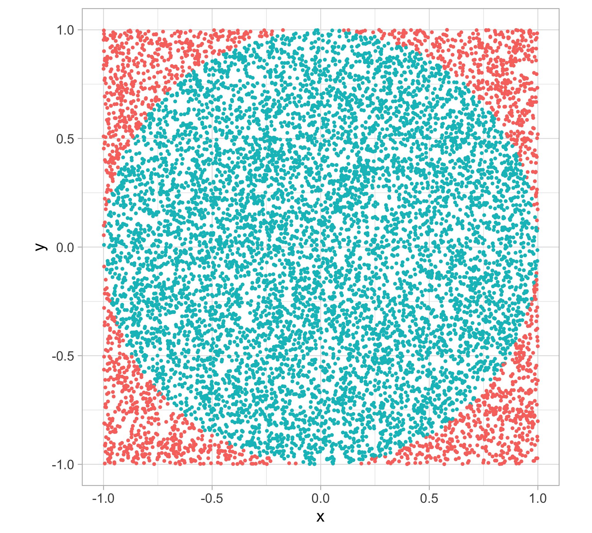
Estimating \(\pi\) using Monte Carlo simulation

• Monte Carlo methods rely on repeated random sampling to obtain numerical results

• Use randomness to solve problems that might be deterministic in principle

• Example: Estimating \(\pi\)

  • Simulate random \((x, y)\) points with domain as a square of side \(2r\) units centered at the origin

  • Consider a circle inside the same domain with same radius \(r\) and inscribed into the square

  • Calculate the ratio of number points inside the circle and total number of generated points (Why?)

Estimating \(\pi\) using Monte Carlo simulation

n_points <- 10000
x <- runif(n_points, -1, 1)
y <- runif(n_points, -1, 1)
inside <- ifelse(x^2 + y^2 <= 1, 1, 0)
4 * mean(inside)

[1] 3.158

tibble(x, y, inside) |> 
  ggplot(aes(x, y, color = factor(inside))) +
  geom_point(show.legend = FALSE) +
  coord_equal()

Pseudorandomness and seeds

Same command, different results?

Not surprisingly, we get different sample draws each time we call rnorm()

mean(rnorm(100))

[1] -0.140778

mean(rnorm(100))

[1] -0.1153921

mean(rnorm(100))

[1] -0.2145186

Is it really random?

Random numbers generated in R (or any language) are not truly random; they are what we call pseudorandom

• These are numbers generated by computer algorithms that very closely mimick truly random numbers

• The default algorithm in R is called the Mersenne Twister

To learn more, type ?Random into R (check out how to change the algorithm used for pseudorandom number generation, which you should never really have to do…)

Setting the random seed

• All pseudorandom number generators depend on what is called a seed value

• This puts the random number generator in a well-defined state, so that the numbers it generates, from then on, will be reproducible

• The seed is just an integer, and can be set with set.seed()

• The reason we set it: so that when someone else runs our simulation code, they can see the same—albeit, still random—results that we do

• Note: set.seed() will be helpful later on for things like cross-validation, \(k\)-means clustering, etc. — basically anything that involves randomly sampling of the data

Setting the random seed

Same seed, same results

set.seed(1999)
rnorm(3)

[1]  0.73267249 -0.03782971  1.20300914

set.seed(1999)
rnorm(3)

[1]  0.73267249 -0.03782971  1.20300914

set.seed(1999)
rnorm(3)

[1]  0.73267249 -0.03782971  1.20300914

Good practices

Repetition and reproducibility

• One single simulation is not always trustworthy (depends on the situation, of course)

• In general, simulations should be repeated and aggregate results reported — requires iteration!

• To make random number draws reproducible, we must set the seed with set.seed()

• More than this, to make simulation results reproducible, we need to follow good programming practices (see this for example)

• Gold standard: any time you show a simulation result (a figure, a table, etc.), you have code that can be run (by anyone) to produce exactly the same result

Iteration and simulation

• Writing a function to complete a single run of your simulation/analysis is often very helpful

• This allows the simulation itself to be intricate (e.g., intricate steps, several simulation parameters), but makes running the simulation simple

• Then you can use iteration to run your simulation/analysis over and over again

Iteration and simulation

Example: Revisiting \(k\)-means clustering with gapminder data - compute the total within-cluster variation for different values of \(k\)

library(dslabs)
clean_gapminder <- gapminder |>
  filter(year == 2011, !is.na(gdp)) |>
  mutate(std_log_gdp = as.numeric(scale(log(gdp), center = TRUE, scale = TRUE)),
         std_life_exp = as.numeric(scale(life_expectancy, center = TRUE, scale = TRUE)))

# function to perform clustering for each value of k
gapminder_kmeans <- function(k) {
  kmeans_results <- clean_gapminder |>
    select(std_log_gdp, std_life_exp) |>
    kmeans(centers = k, nstart = 30)
  
  kmeans_out <- tibble(clusters = k,
                       total_wss = kmeans_results$tot.withinss)
  return(kmeans_out)
}

# number of clusters to search over
n_clusters_search <- 2:12

# iterate over each cluster value to compute total wss
kmeans_search <- n_clusters_search |> 
  map(gapminder_kmeans) |> 
  bind_rows()

Pre-allocation

Example: When 100 coins are tossed, what is the probability that exactly 50 are heads?

library(tictoc)
n_runs <- 500000
a <- c()
tic()
for (i in 1:n_runs) {
  tosses <- sample(0:1, size = 100, replace = TRUE)
  a[i] <- sum(tosses)
}
toc()

b <- rep(NA, n_runs)
tic()
for (i in 1:n_runs) {
  tosses <- sample(0:1, size = 100, replace = TRUE)
  b[i] <- sum(tosses)
}
toc()

# exact: (factorial(100) / (factorial(50) * factorial(50))) * (1 / 2) ^ 100
mean(b == 50)

Pre-allocation

• Not only computations take time, memory allocations do too

• Changing the size of a vector takes just about as long as creating a new vector does

• Each time the size changes, R needs to reconsider its allocation of memory to the object

• Never reallocate a vector after each iteration

Analogy

Exporting and importing data

Reading/writing from/to a file

Sometimes simulations/analyses take a long time to run, and we want to save intermediate or final output, for quick reference later

Introducing the readr package (part of tidyverse; automatically loaded)

• write_*() functions: exporting data

• read_*() functions: importing data

Reading/writing from/to a file

• write_csv() / read_csv(): export / import single R data frames or tibbles in .csv format

• write_rds() / read_rds(): export / import single R objects (like a vector, matrix, list, data frame, etc.) in .rds format

Note that by default, the file will be written to the working directory (i.e. if you just specify the file name)

example_df <- tibble(x = rnorm(100), y = rnorm(100))
write_rds(example_df, "INSERT PATH/example_df.csv")
df <- read_csv("INSERT PATH/example_df.csv")

example_obj <- matrix(rnorm(25), 5, 5)
write_rds(example_obj, "INSERT PATH/example_obj.rds")
obj <- read_rds("INSERT PATH/example_obj.rds")

Example: saving \(k\)-means clustering results from earlier

# saving to a folder named "data" in the working directory
write_csv(kmeans_search, "data/kmeans_search_results.csv")

File path and working directory

• To read in a file, you need to use the correct path, which should be relative and NOT absolute (or a path pointing to a location outside of the project directory) (read more here)

• The key to getting paths to work is to understand working directory. In R, use the function getwd()

  • Note: NEVER use setwd() to change working directory. (Here’s why)

• Naming things (files, folders, etc.): see here and here

File path and working directory

• Special paths

  • . is the working directory

  • ~ is the home directory (e.g., on Quang’s laptop: /Users/qntkhvn)

  • .. is the parent directory. (e.g., ../steve.csv refers to a file called steve.csv in the directory that is one level above the working directory)

• Common issue

  • By default, the working directory for an R Markdown or Quarto document is the directory in which that document is stored.

  • This is NOT necessarily the working directory of your current R session.

• Use list.files() to see what files are available in the working directory (or any other directory)

list.files()
list.files("~")

Resources

• here package

• fertile package

• What They Forgot to Teach You About R

In reality…