Supervised learning: linear regression
Visual explanation
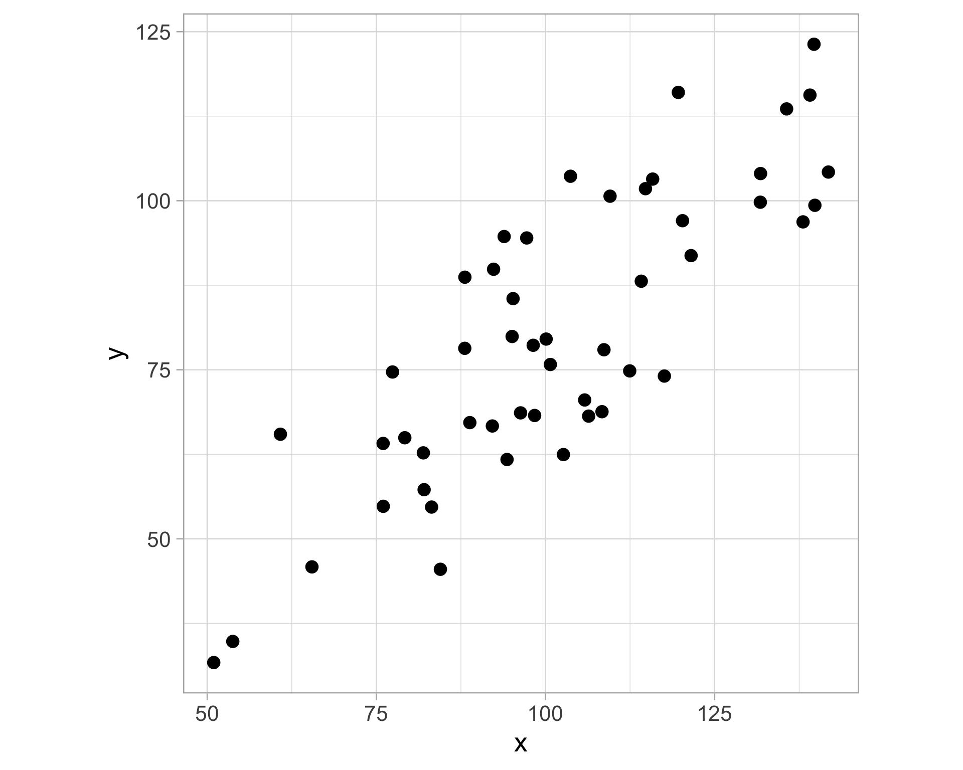
Imagine a 2D scatterplot with different data points
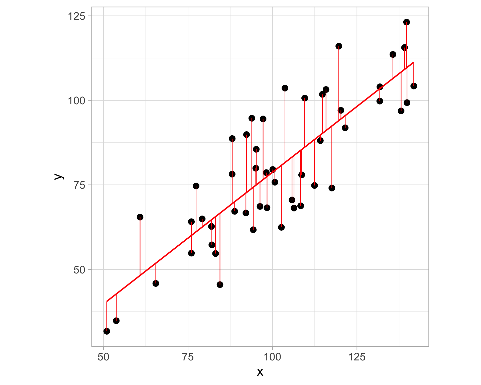
Linear regression aims to find a “best fit” line that minimizes the vertical distance between the line and the data points
- The vertical distance is known as a residual (difference between the actual y-value of a data point and the predicted y-value on the regression line)
Modeling bike ridership
To best serve its members, Capital Bikeshare must understand the demand for its service
Modeling & predicting bikeshare
rides
bikes |>
  ggplot(aes(x = rides)) +
  geom_histogram(color = "black", fill = "gray")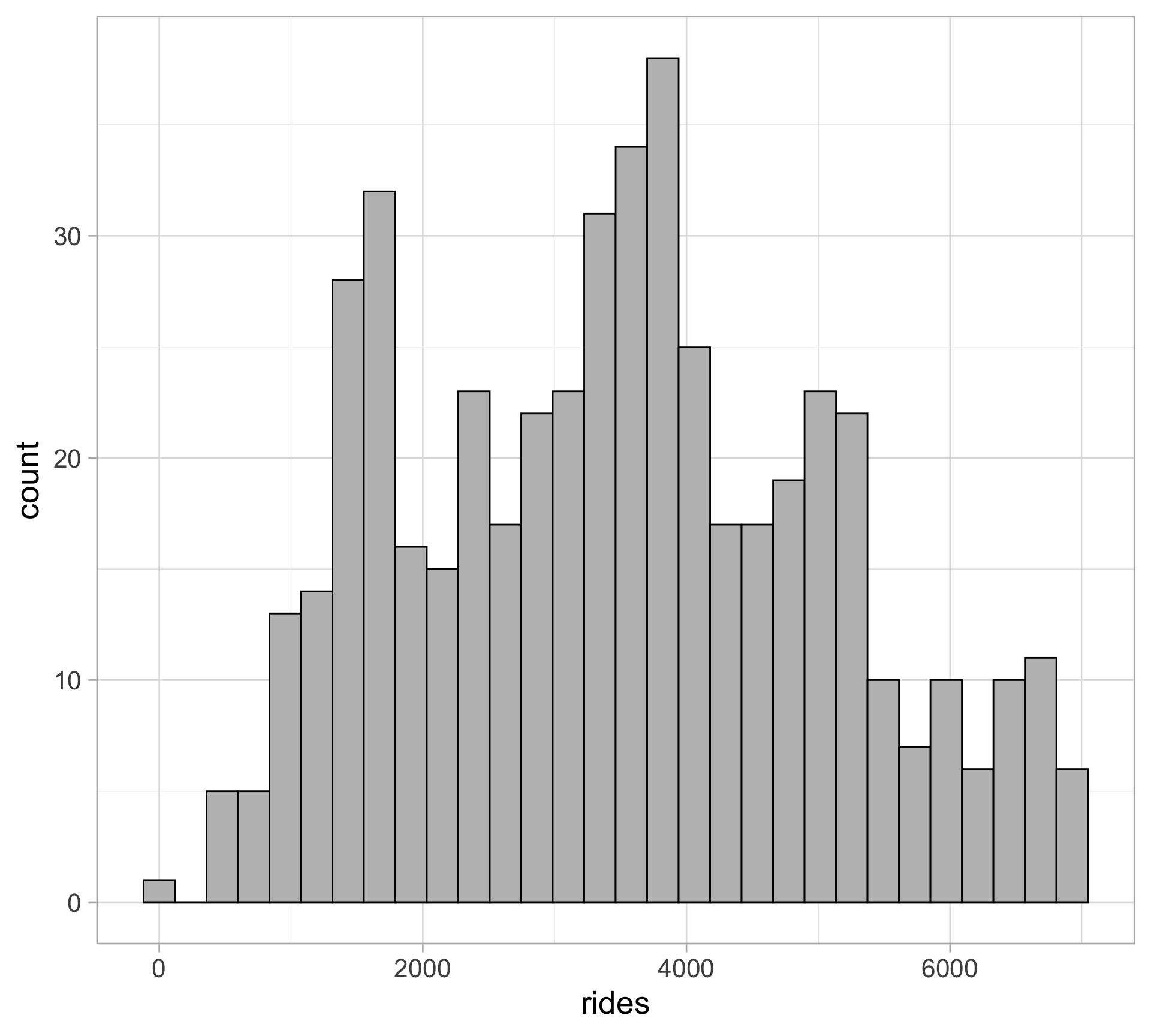
Relationship between rides and feels-like temperature
rides_temp <- bikes |>
  ggplot(aes(x = temp_feel, y = rides)) +
  geom_point(size = 3, alpha = 0.5)
rides_temp
We fit linear regression models using lm(), formula is input as: response ~ predictor
simple_lm <- lm(rides ~ temp_feel, data = bikes) 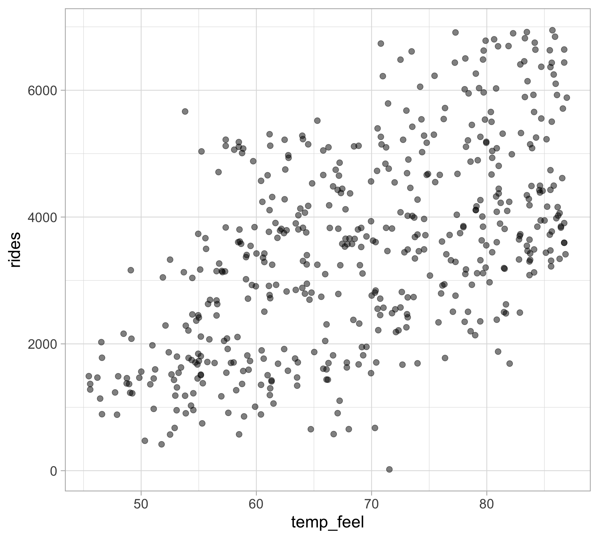
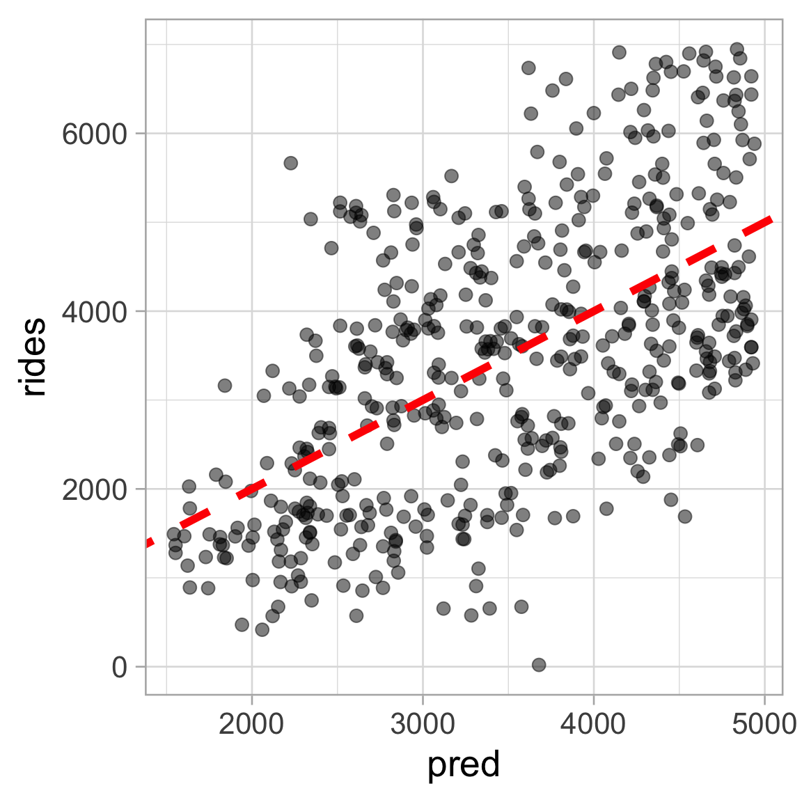
Plot observed values against predictions
Useful diagnostic (for any type of model, not just linear regression!)
bikes |>
  mutate(pred = predict(simple_lm)) |>
  ggplot(aes(x = pred, y = rides)) +
  geom_point(alpha = 0.5, size = 3) +
  geom_abline(slope = 1, intercept = 0,
              linetype = "dashed",
              color = "red",
linewidth = 2)- “Perfect” model will follow diagonal
Plot observed values against predictions
Augment the data with model output using the broom package
augment() adds various columns from model fit we can use in plotting for model diagnostics
bikes <- simple_lm |>
  augment(bikes)
bikes |>
  ggplot(aes(x = .fitted, y = rides)) +
  geom_point(alpha = 0.5, size = 3) +
  geom_abline(slope = 1, intercept = 0, color = "red",
              linetype = "dashed", linewidth = 2)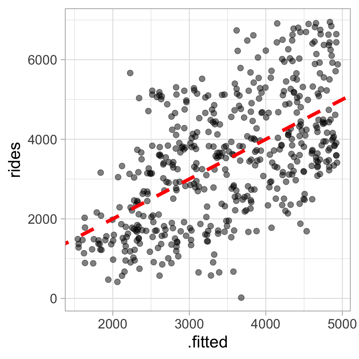
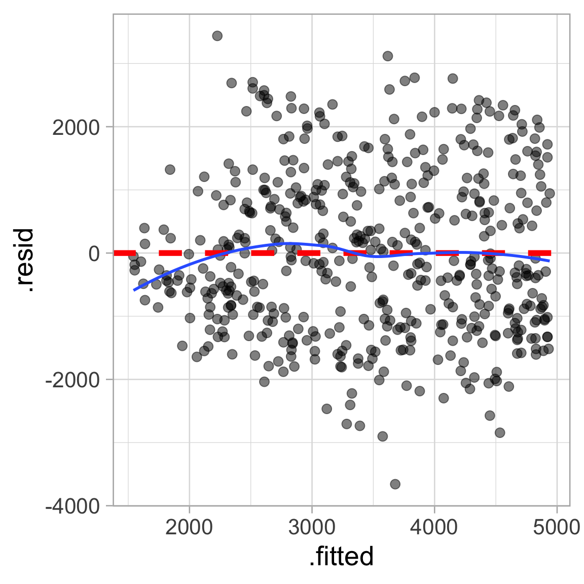
Plot residuals against predicted values
Residuals = observed - predicted
Interpretation of residuals in context?
Conditional on the predicted values, the residuals should have a mean of zero
bikes |>
  ggplot(aes(x = .fitted, y = .resid)) +
  geom_point(alpha = 0.5, size = 3) +
  geom_hline(yintercept = 0, linetype = "dashed",
             color = "red", linewidth = 2) +
  # plot the residual mean
  geom_smooth(se = FALSE)
Residuals should NOT display any pattern
Two things to look for:
Any trend around horizontal reference line?
Equal vertical spread?
Comparing observed values and predictions
Similar to before, we can plot the actual and predicted ridership
To reiterate, all we’re doing is changing the intercept of our regression line by including a categorical variable
bikes |>
  mutate(season_pred = predict(season_lm)) |>
  ggplot(aes(x = rides, y = season_pred)) +
  geom_point(size = 3, alpha = 0.5) +
  facet_wrap(~ season, ncol = 4) +
  labs(x = "Actual number of rides",
       y = "Predicted number of rides")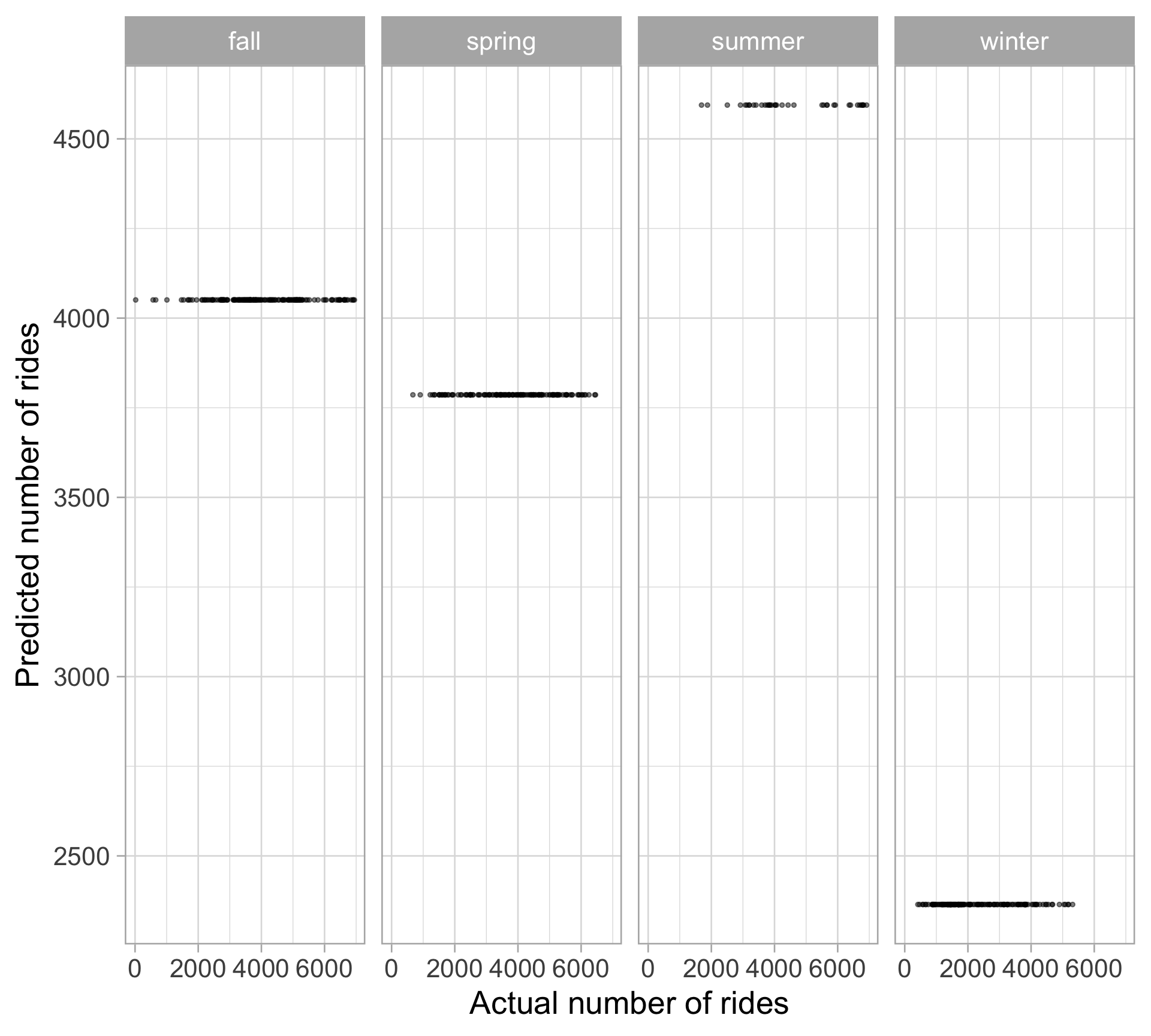
Visualizing interactions
bikes |>
  ggplot(aes(x = temp_feel, y = rides, color = season)) +
  geom_point(size = 2, alpha = 0.6) +
  geom_smooth(method = "lm", se = FALSE, linewidth = 2) +
  ggthemes::scale_color_colorblind()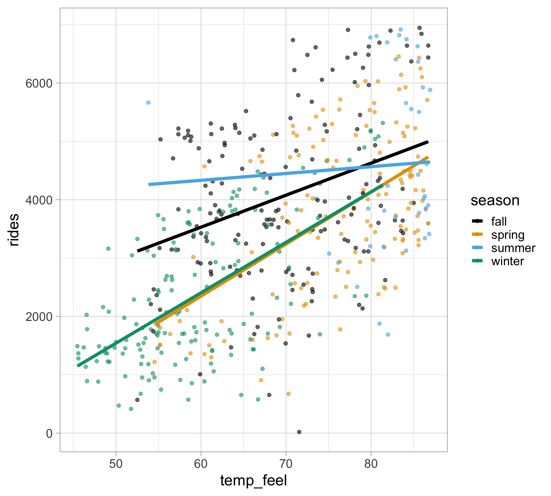
Regression confidence intervals
geom_smooth()displays confidence intervals for the regression line
# predict(simple_lm, interval = "confidence")
lm_plot <- bikes |>
  ggplot(aes(x = temp_feel, y = rides)) +
  geom_point(alpha = 0.5) +
  geom_smooth(method = "lm")
lm_plot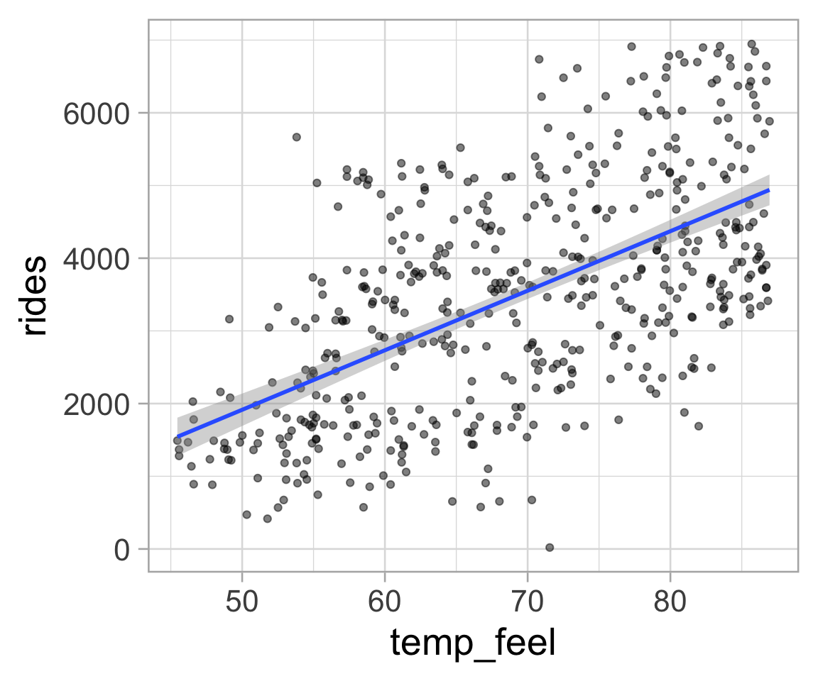
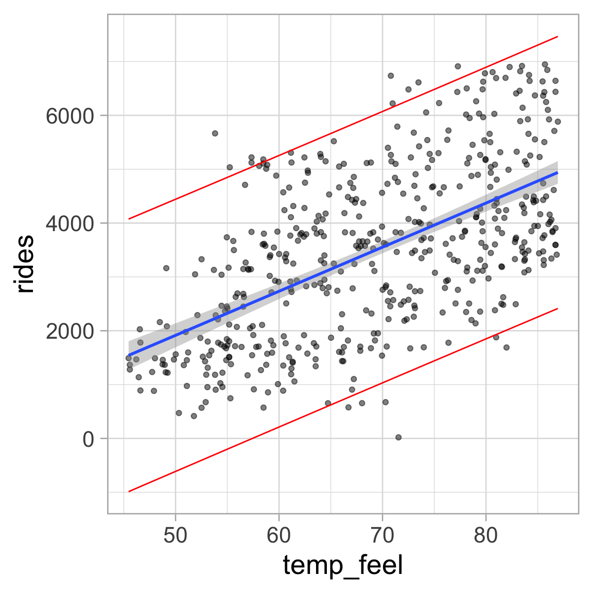
Confidence intervals versus prediction intervals
Generate 95% intervals
# predict(simple_lm, interval = "prediction")
lm_plot +
  geom_ribbon(
    data = augment(simple_lm, interval = "prediction"),
    aes(ymin = .lower, ymax = .upper),
    color = "red", fill = NA
  )
The standard error for predicting an individual response will always be larger than for predicting a mean response
Prediction intervals will always be wider than confidence intervals