Supervised learning: model building

SURE 2025

Department of Statistics & Data Science
Carnegie Mellon University

Variable selection

Old school approaches (not recommended)

Best subset selection
Forward/backward/stepwise selection

Limitations
- only feasible for a smaller number of variables
- computationally infeasible for a large number of predictors
- arbitrary way of defining the best model and ignores contextual knowledge about potential predictors

Variable selection is a difficult problem!

Like much of a statistics research, there is not one unique, correct answer

Do not turn off your brain! Algorithms can be tempting but they are NOT substitutes!

Justify which predictors used in modeling based on:
- domain knowledge
- extensive EDA
- model assessment based on holdout predictions (w/ cross-validation, we’ll discuss this in a bit)

Be a responsible modeler! (Check out this substack)

Confounding variables

A confounding variable (or lurking variable) is one that is associated with both the response and predictor variables

It can be tempting to immediately jump to conclusions when faced with a strong association between the variables
However, it is important to stop and think about whether there are confounding variables which could be explaining the association instead

Confounding variables

In studying the relationship between a predictor \(X\) and a response variable \(Y\),

We should adjust for confounding variables that can influence that relationship because they are associated both with \(X\) and with \(Y\)
If the variable is a potential confounder, including it in the model may help to reduce bias in estimating relevant effects of key explanatory variables

Confounding variables

Example: Examine the impact of fertilizer on the yield of an apple orchard

Suppose researchers are studying the relationship between the amount of fertilizer used and the yield of apple orchards

They fit a model with the yield as the response and amount of fertilizer used as the single predictor

But, there are many possible confounding variables that might be associated with both the amount of fertilizer used and the yield (e.g., quality of soil, weather, etc.)

These variables, if included in the data, should also be adjusted for in the model

Just remember…

Conditioning is the soul of statistics. — Joe Blitzstein

The trade-offs

Which model(s) should I use in my analysis?

The answer: IT DEPENDS

Setup: Let \(Y\) be the response variable, and \(X = (X_1, X_2, \dots, X_p)\) be the predictors
- We want to fit a model to estimate an unknown function \(f\) describing the relationship between \(Y\) and \(X\)
- The learned model will take the form \(\hat{Y}=\hat{f}(X)\)

What is the goal of your modeling problem?
- If you care more about the details of \(\hat{f}(X)\), then it’s an inference problem
- If you care more about predictive power, then it’s a prediction problem

Any algorithm can be used for prediction, however options are limited for inference

Active area of research: inference for black box models

Some trade-offs

Model flexibility vs interpretability
- Linear models are easy to interpret; boosted trees are not

Good fit vs overfit or underfit
- How do we know when the fit is just right?

Parsimony vs black-box
- A simpler model with fewer variables vs a black-box involving more (or all) predictors?

Model flexibility vs interpretability

Generally speaking: trade-off between a model’s flexibility (i.e. how “wiggly” it is) and how interpretable it is

Parametric methods: we make an assumption about the functional form, or shape, of \(f\) before observing the data

Nonparametric methods: we do not make explicit assumptions about the functional form of \(f\) (i.e., \(f\) is estimated from the data)

Parametric models are generally easier to interpret, whereas nonparametric models are more flexible

If your goal is prediction, your model can be as arbitrarily flexible as it needs to be (but be careful…)

If your goal is inference, there are clear advantages to using simpler and more interpretable models

Measuring the quality of model fit

Suppose we fit a model to some training data and we wish to see how well it performs

In the regression setting, we could compute the mean squared error (MSE) over the training set \[\text{MSE}_{\texttt{train}} = \frac{1}{n} \sum_{i \in \texttt{train}} (y_i - \hat f(x_i))^2\]

But this may be biased toward more overfit models

Instead, we should compute the MSE using previously unseen test (holdout) data (i.e. data not used to train the model) to ensure generalizability \[\text{MSE}_{\texttt{test}} = \frac{1}{n} \sum_{i \in \texttt{test}} (y_i - \hat f(x_i))^2\]

MSE is an example of a loss/objective/cost function—a performance measure that represents the quality of a model fit

Model flexibility and assessment example

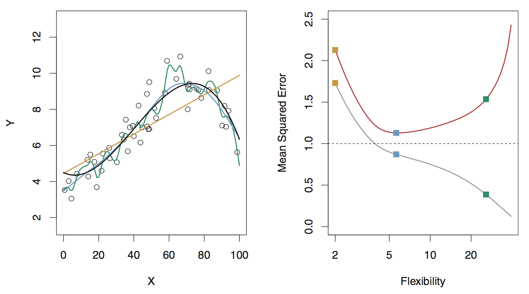
Black curve (left): truth

Orange, blue and green curves/squares: fits of different flexibility

Gray curve (right): \(\text{MSE}_{\texttt{train}}\). Red curve (right): \(\text{MSE}_{\texttt{test}}\)

Model flexibility and assessment example

Black curve (left): true model

Data are generated from a smoothly varying non-linear model with random noise added

Model flexibility and assessment example

Orange line (left): linear regression fit: inflexible, fully parametrized, underfitting

Green curve (left): an overly flexible, nonparametric model: overfits (follows noise too closely)

Blue curve (left): aims to strike a balance, not too smooth, not too wiggly.

Model flexibility and assessment example

Gray line (right): training error (MSE) decreases as flexibility increases.

Red line (right): test error (MSE) decreases until a “sweet spot”, then increases due to overfitting

Bias-variance trade-off

Typical trend
- Underfitting means high bias & low variance (fitting a line to the data)
- Overfitting means low bias & high variance (drawing a wiggly curve that passes through every single training observation)

Generally, as the flexibility of a model fit increases, its variance increases, and its bias decreases

So choosing the flexibility based on average test error amounts to a bias-variance trade-off

Bias-variance trade-off

Orange curve/squares (linear model): high bias, low variance

Green curve/squares (overly flexible model): low bias, high variance

Blue curve/squares: optimal (“just right”) amount of flexibility is somewhere in the middle

Bias-variance trade-off: thought experiments

Can we ever predict \(Y\) from \(X\) with zero error?

Generally, no… even the true \(f\) cannot generically do this, and will incur some error due to noise
This is called the irreducible error \(\epsilon\)

What happens if our fitted model \(\hat f\) belongs to a model class that is far from the true \(f\)?

For example, we fit a linear model in a setting where the true relationship is far from linear
As a result, we encounter a source of error: estimation bias

What happens if our fitted model \(\hat f\) is itself quite variable?

In other words, over different training sets, we end up constructing substantially different \(\hat f\)
This is another source of error: estimation variance

Bias-variance decomposition

The expected test error, conditional on \(X = x\) for some \(x\), can be decomposed as \[\mathbb E[(Y - \hat f(x))^2 \mid X = x] = \text{Bias}^2[\hat f(x)] + \text{Var}[\hat f(x)] + \text{Var}[\epsilon]\]

In order to minimize the expected test error, we need a model that simultaneously achieves low variance and low bias

But, the variance is a nonnegative quantity, and squared bias is also nonnegative

Thus, there’s a trade-off between bias and variance
- Even if our prediction is unbiased, we can still incur a large error if it is highly variable
- Meanhile, even when our prediction is stable and not variable, we can incur a large error if it is badly biased

“The sweet spot”

Remember, when building predictive models, try to find the sweet spot between bias and variance. #babybear
— Dr. G. J. Matthews (@StatsClass) September 6, 2018

Check out this song

Principle of parsimony (Occam’s razor)

“Numquam ponenda est pluralitas sine necessitate” (plurality must never be posited without necessity)

From ISLR:

When faced with new data modeling and prediction problems, it’s tempting to always go for the trendy new methods. Often they give extremely impressive results, especially when the datasets are very large and can support the fitting of high-dimensional nonlinear models. However, if we can produce models with the simpler tools that perform as well, they are likely to be easier to fit and understand, and potentially less fragile than the more complex approaches. Wherever possible, it makes sense to try the simpler models as well, and then make a choice based on the performance/complexity trade-off.

In short: “When faced with several methods that give roughly equivalent performance, pick the simplest.”

The curse of dimensionality

The more features, the merrier?… Not so fast, my friend.

Adding additional signal features that are truly associated with the response will improve the fitted model
- Reduction in test set error

Adding noise features that are not truly associated with the response will lead to a deterioration in the model
- Increase in test set error
- Noise features increase the dimensionality of the problem, exacerbating the risk of overfitting
- (Noise features may be associated with the response on the training set due to chance)

Cross-validation

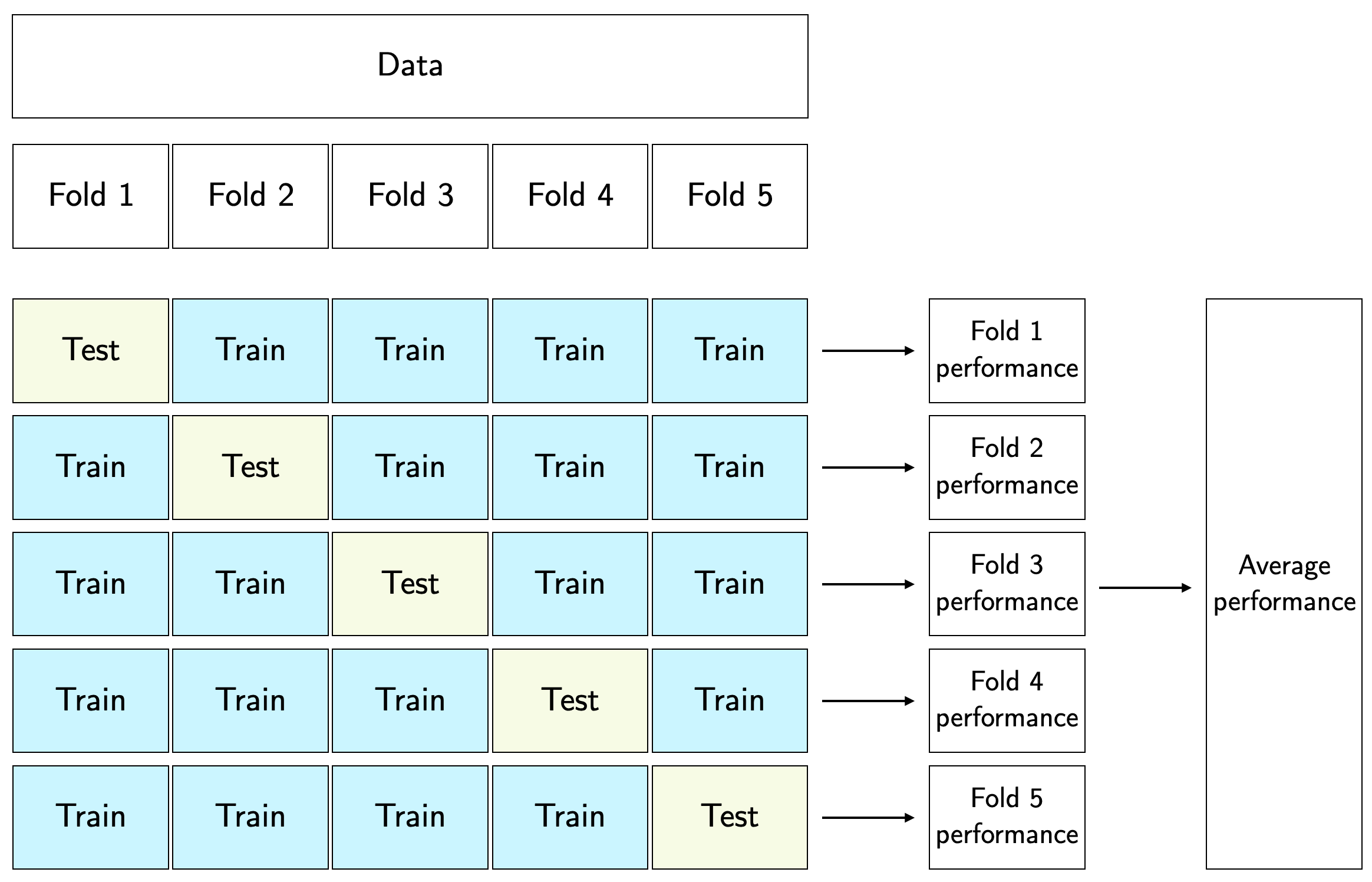
\(K\)-fold cross-validation

Randomly split the observations into \(K\) (roughly) equal-sized folds (usually \(K=5\) or \(K=10\))

For each fold \(k=1,2,\dots,K\)
- Fit the model on data excluding observations in fold \(k\)
- Obtain predictions for fold \(k\)
- Compute performance measure (e.g. MSE) for fold \(k\)

Aggregate performance measure across folds
- e.g., compute average MSE, including standard error

We can justify model choice (e.g. model selection/comparison, variable selection, tuning parameter selection) using any performance measure we want with CV

Why do we typically choose \(K=5\) or \(K=10\)? Think about: What’s the smallest and largest \(K\) could be? And what’s the trade-off?

(5-fold) cross-validation procedure diagram

Some notes on cross-validation

Recall that the typical cross-validation procedure randomly assigns individual observations to different folds

In more complex data settings (e.g. correlated data, nested data), figuring out the appropriate way to split the observations into folds can require careful thoughts

For example, if the data are spatially or temporally dependent, we can’t simply assign individual observations to folds (which may result in data leakage)

To preserve any dependence structure of the data, we can assign groups/blocks of observations together into different folds

Cross-validation example: model comparison

Data on Capital Bikeshare, similar to linear regression lecture

library(tidyverse)
theme_set(theme_light())
bikes <- read_csv("https://raw.githubusercontent.com/36-SURE/2025/refs/heads/main/data/bikes.csv")

Compare the following model for predicting number of bikeshare rides
- Model 1: includes only 1 predictor–feels like temperature
- Model 2: includes 2 predictors–feels like temperature and season
- Model 3: same as model 2, but adding the interaction between temperature and season

Assigning observations to fold

Perform 5-fold cross-validation to assess model performance
Create a column of test fold assignments to our dataset with the sample() function
Always remember to set.seed() prior to performing cross-validation

set.seed(100)
N_FOLDS <- 5
bikes <- bikes |>
  mutate(fold = sample(rep(1:N_FOLDS, length.out = n())))
# table(bikes$fold)

Model comparison based on out-of-sample performance

Function to perform cross-validation

bikes_cv <- function(x) {
  
  # get test and training data
  test_data <- bikes |> filter(fold == x)                     
  train_data <- bikes |> filter(fold != x)
  
  # fit models to training data
  interaction_fit <- lm(rides ~ temp_feel * season, data = train_data)
  temp_season_fit <- lm(rides ~ temp_feel + season, data = train_data)
  temp_fit <- lm(rides ~ temp_feel, data = train_data)
  
  # return test results
  out <- tibble(
    interaction_pred = predict(interaction_fit, newdata = test_data),
    temp_season_pred = predict(temp_season_fit, newdata = test_data),
    temp_pred = predict(temp_fit, newdata = test_data),
    test_actual = test_data$rides,
    test_fold = x
  )
  return(out)
}

bikes_test_preds <- map(1:N_FOLDS, bikes_cv) |> 
  bind_rows()

Model comparison based on out-of-sample performance

Compute RMSE across folds with standard error intervals

bikes_test_summary <- bikes_test_preds |>
  pivot_longer(interaction_pred:temp_pred, names_to = "model", values_to = "test_pred") |>
  group_by(model, test_fold) |>
  summarize(rmse = sqrt(mean((test_actual - test_pred)^2)))

bikes_test_summary |> 
  group_by(model) |> 
  summarize(avg_cv_rmse = mean(rmse),
            sd_rmse = sd(rmse),
            k = n()) |>
  mutate(se_rmse = sd_rmse / sqrt(k),
         lower_rmse = avg_cv_rmse - se_rmse,
         upper_rmse = avg_cv_rmse + se_rmse) |> 
  select(model, avg_cv_rmse, lower_rmse, upper_rmse)

# A tibble: 3 × 4
  model            avg_cv_rmse lower_rmse upper_rmse
  <chr>                  <dbl>      <dbl>      <dbl>
1 interaction_pred       1242.      1216.      1269.
2 temp_pred              1288.      1261.      1316.
3 temp_season_pred       1239.      1211.      1268.

Visualizing model performance results

bikes_test_summary |> 
  ggplot(aes(x = model, y = rmse)) + 
  geom_point(size = 4) +
  stat_summary(fun = mean, geom = "point", 
               color = "red", size = 4) + 
  stat_summary(fun.data = mean_se, geom = "errorbar", 
               color = "red", width = 0.2)

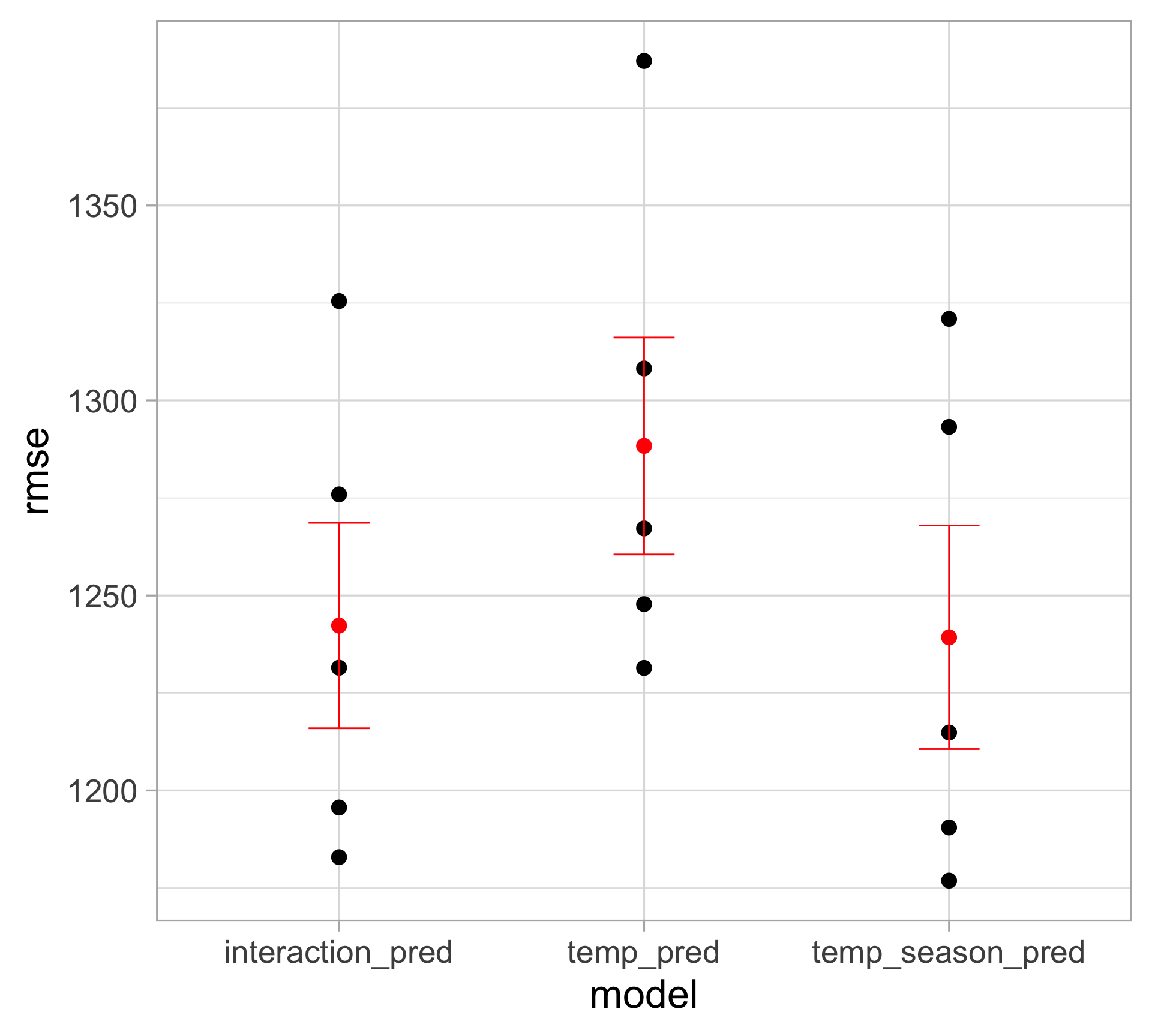
Including season (together with temperature) clearly provides better performance
Including an interaction term between season and temperature is not worthwhile
(in fact, the performance is slightly worse compared to the model without interaction)

Model building checklist

Before doing any modeling/analysis…

Think carefully about what the ideal data would be
- Do you have the suitable data?
- What is the appropriate data format for the modeling problem?

Write down different aspects you want your model to capture
- Distribution of the response?
- Different types of feature?
- Any dependence structure you want your model to capture?
- …

Make sure to justify the model choice

Why is your model appropriate for the problem?

For simplicity and explanability purpose? (Why do you prefer a simpler model over a black box?)
For complexity and flexibility purpose? (Why do you prefer a black box over a simpler model?)

How do you evaluate your model?

Do you compare it with other models? Do you have a baseline model?
Do you compare it with alternative specifications (e.g. different set of predictors)?

How do you choose the predictors?

domain knowledge?
extensive EDA?
model assessment based on holdout predictions?

Make sure to report uncertainty for whatever you’re estimating

Don’t just say “we find a statistically significant association between Y and X…”

What do those coefficient estimates tell you? Interpret in context
How large/small is the effect size?
What’s the margin of error?
Did the model also adjust for other potential meaningful predictors?

This also applies to (\(k\)-fold) cross-validation results

Report the average of the performance measure (e.g. MSE, accuracy, etc.) across the \(k\) test set along with standard errors
In some cases, all \(k\) folds yield similar results, but in other cases, the results are vastly different across the folds
Without some indication of uncertainty, no one will have a clue of how reliable your results are