
Data wrangling with R’s data.table package
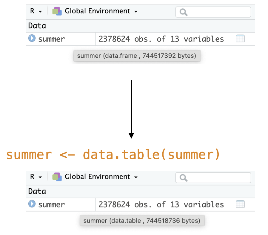
What is data.table?
A versatile R package that is a high performance version of base R’s
data.frame.1Benefits include:
Computational efficiency
Concise syntax
No dependencies
Tested against old versions of R
Uses: data wrangling, reading/writing files, handling large data, and much more!
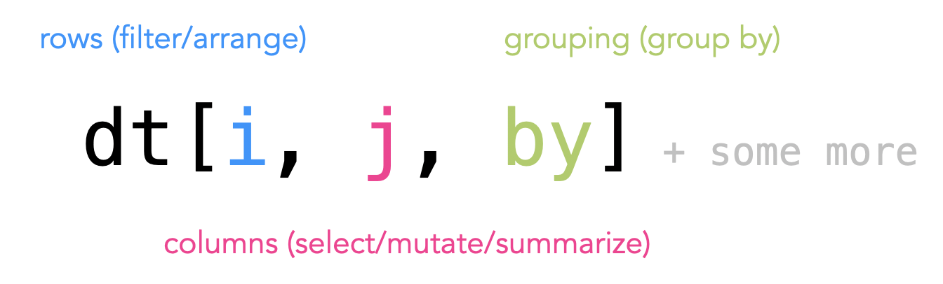
data.table syntax
The six main verbs all follow a three part syntax:
Example data
pets_dtis collected on students who have one petpet: animal student hasn_classes: number of classes the student ishours_hw: hours of homework the student has
pets_dt <- rowwiseDT(pet =, n_classes=, hours_hw=,
                    "cat", 3, 18,
                    "dog", 4, 24,
                    "fish", 2, 10,
                    "dog", 3, 12,
                    "dog", 1, 8,
                    "cat", 1, 3,
                    "fish", 4, 16,
                    "fish", 1, 6)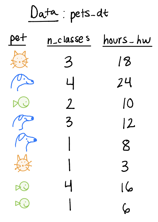
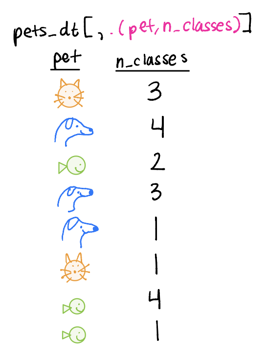
Selecting columns
We can select columns to keep in our dataset
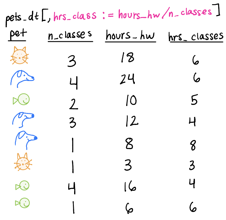
Mutating variables
We can add (mutate) variables to the dataset, keeping the same number of rows as before
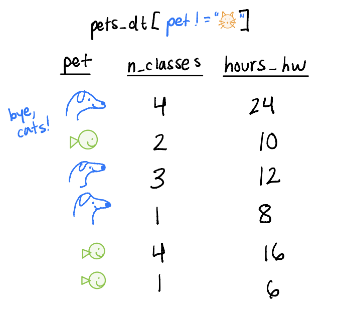
Filtering rows
We can filter for particular type of row based on a logical statement
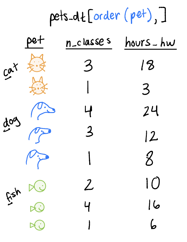
Arranging rows
We can arrange the dataset by a particular variable(s)
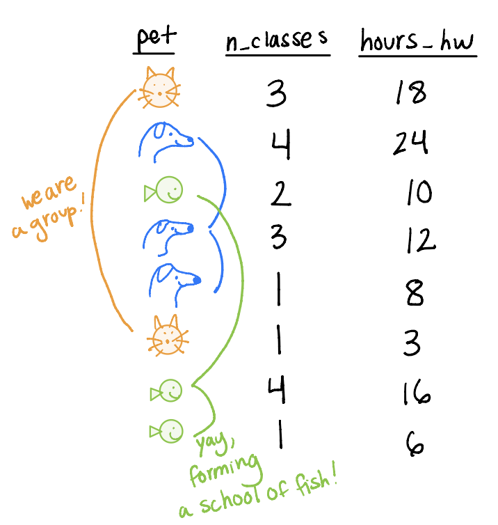
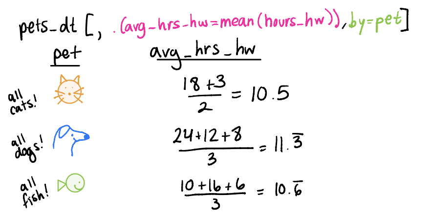
Grouping by and summarizing
We can create summary statistics (summarize) by particular groups (group_by)
Let’s poll!

Joining datasets
We might also want to join two datasets, meaning we combine them based on the information in each respective one.
In data.table, joins are supported by the base syntax:
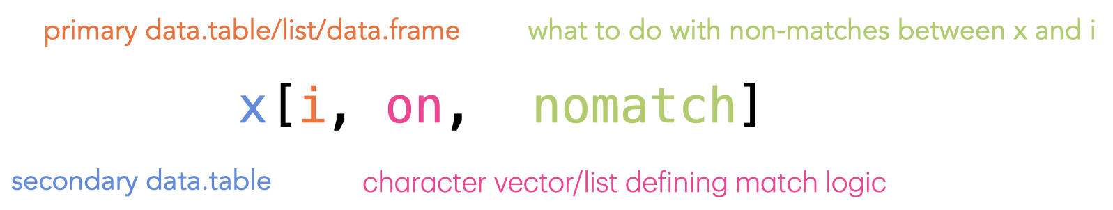
Note that joins are right joins by default in data.table!
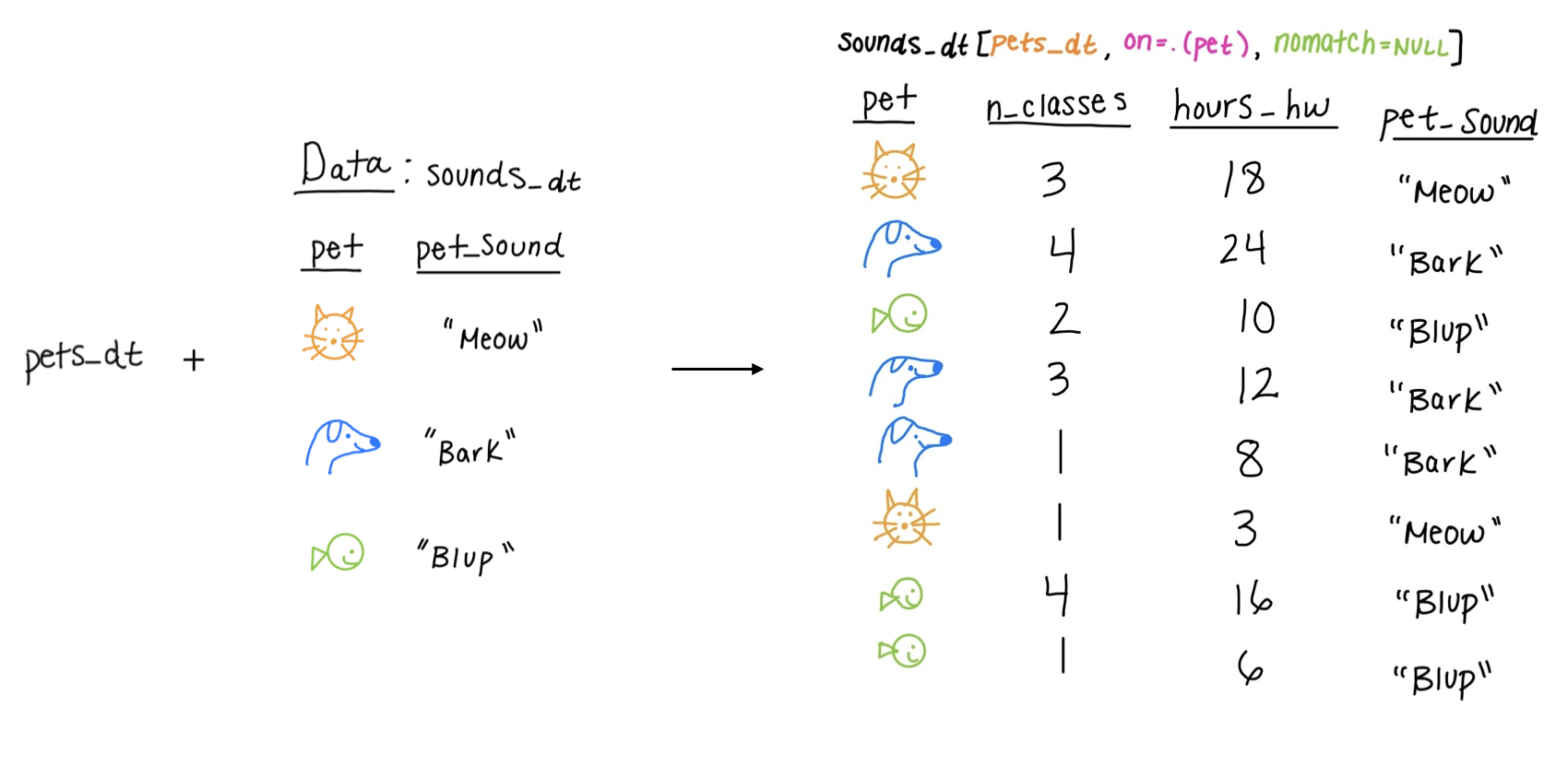
Equi joins
Equi joins: find common elements between the two datasets to combine
Inner Join Example:
Piping statements together
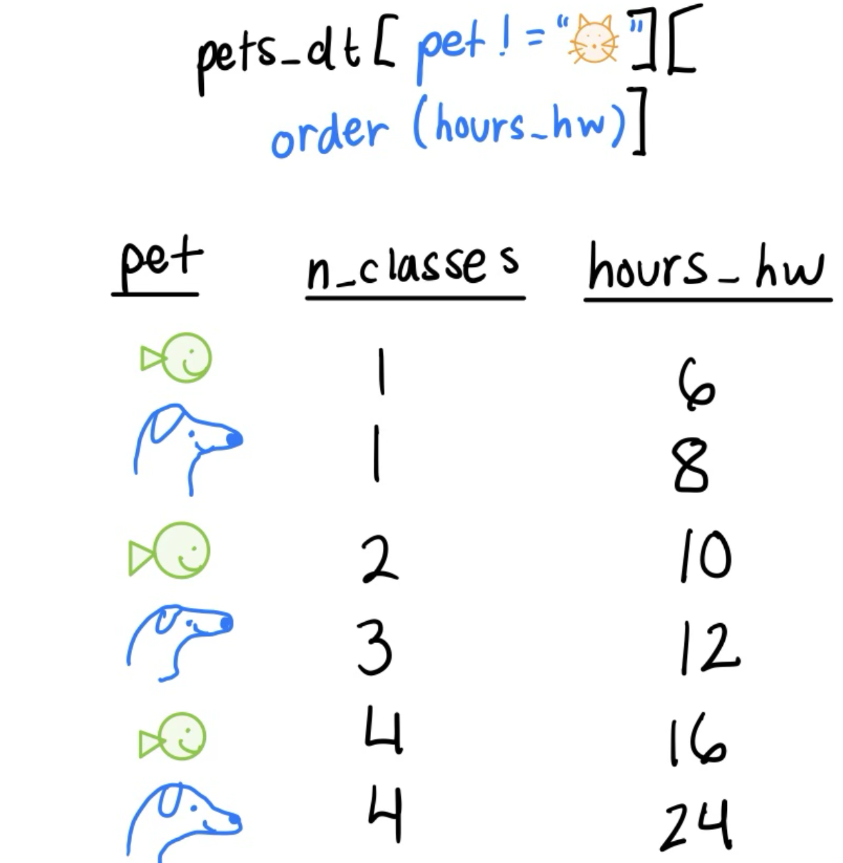
What if we wanted to pair multiple of the six main verbs together? For example, filter pets_dt to remove the cats and then arrange by hours_hw?
- We could save the filtered dataset to
no_cats_dtand then order that. - We could also pipe statements together!
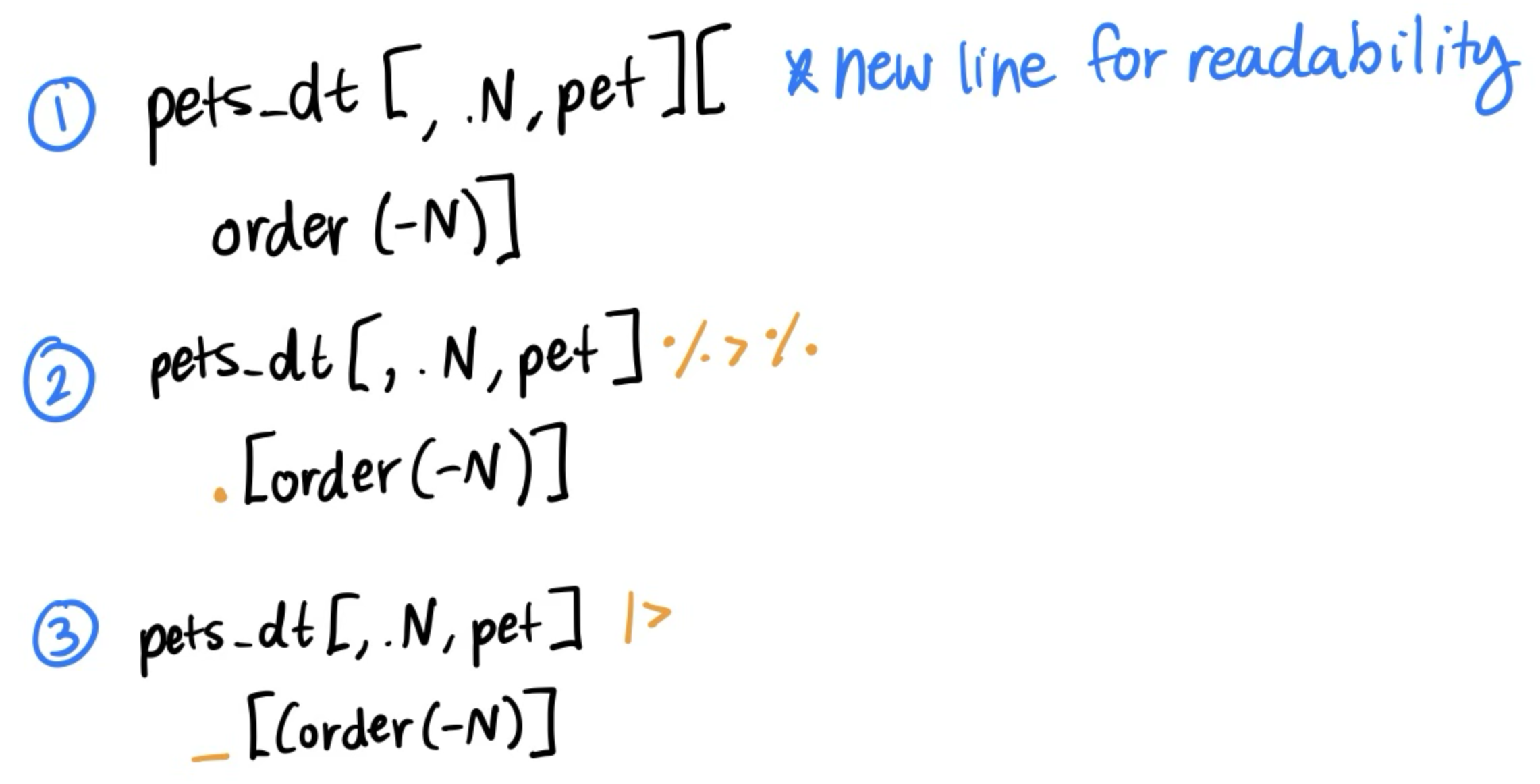
Three equivalent ways to pipe
Visualizing by a grouping variable
Let’s say we are investigating the relationship between lot area and sale price and we want to see how it varies by driveway pavement.
house_prices[, print(
  ggplot(.SD, aes(x=Lot.Area, y=SalePrice))+
    geom_point(alpha=0.5)+
    theme_classic()+
    ggtitle(paste("Paved.Drive:", Paved.Drive[1]))), by=.(Paved.Drive)]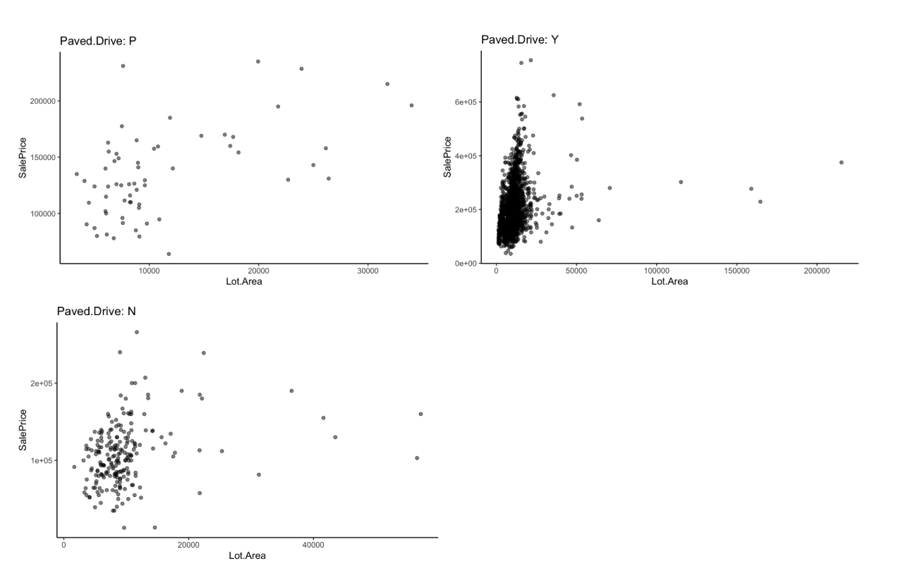
Weighing the options
- Both
data.tableandtidyverseare great tools for wrangling data. Luckily, we are not confined to just one of them!1 - It all comes down to personal preference:
- Comfort with syntax
- Brevity of syntax
- Consistency with collaborators
- Computational efficiency 2
So, what do we mean when we say data.table is computationally efficient?

Post-Lecture Survey