Supervised learning: generalized linear models


SURE 2025

Department of Statistics & Data Science
Carnegie Mellon University

Background

Recap

  • When the response is continuous, we can use linear regression
  • When the response is binary categorical, we can use logistic regression
  • Which model do we use if the response contains discrete counts?

Generalized linear models (GLMs)

Three components of a GLM

1. Random component (distribution of the response)

  • Identifies the response variable and assumes a probability distribution for it

2. Linear predictor

  • Specifies the predictor variables

  • Linear combination of predictors on the right-hand side of the model equation

  • In the form \(\beta_0 + \beta_1 X_1 + \dots + \beta_p X_p\)

3. Link function (a function of the parameter)

  • Connects the random component with the linear predictor

  • Via a function of the expected value of the probability distribution of the response

See also: Exponential family

Linear regression

  1. \(Y \sim N(\mu, \sigma ^2)\)
  1. Linear predictor: \(\beta_0 + \beta_1 X_1 + \dots + \beta_p X_p\)
  1. Identity link function: \(g(\mu) = \mu\)

Logistic regression

  1. \(Y \sim \text{Binomial}(n,p)\)
  1. Linear predictor: \(\beta_0 + \beta_1 X_1 + \dots + \beta_p X_p\)
  1. Logit link function: \(\displaystyle g(p) = \log\left(\frac{p}{1-p}\right)\)

(Recall: We cannot just simply model \(p = \beta_0 + \beta_1 X_1 + \dots + \beta_p X_p\) since the binary response can only take on values of either 0 or 1)

Poisson regression

  1. \(Y \sim \text{Poisson}(\lambda)\)
  1. Linear predictor: \(\beta_0 + \beta_1 X_1 + \dots + \beta_p X_p\)
  1. Log link function: \(\displaystyle g(\lambda) = \log (\lambda)\)

(We cannot just simply model \(\lambda = \beta_0 + \beta_1 X_1 + \dots + \beta_p X_p\) since the counts can only take on non-negative integers)

Generalization example

In linear regression, the distribution is normal and the domain of \(Y \mid x\) is \((-\infty,\infty)\)

What, however, happens if we know that

  • the domain of observed values of the response is actually \([0,\infty]\)

  • the observed values are discrete, with possible values \(0, 1, 2, \dots\)

The normal distribution doesn’t hold here

  • Which distribution could possibly govern \(Y \mid x\)?

  • Remember, we might not know truly how \(Y \mid x\) is distributed, but any assumption we make has to fit with the nature of the data

Generalization: Poisson regression

  • PMF of a Poisson distribution: \(\displaystyle f(x \mid \lambda)= \frac{ e^{-\lambda} \lambda^x}{x!}\); \(x = 0, 1, 2, \dots\) and \(\lambda > 0\)
  • Model for the counts of an event in a fixed period of time or space, with a rate of occurrence (intensity) parameter \(\lambda\)
  • \(\lambda\) is both the mean and the variance of the distribution

    • in general, the variance governs the distribution’s shape
  • distribution of independent event occurrences in an interval, e.g. soccer goals in a match

  • \(\lambda\) is the average number of the events in an interval

So, when we apply GLM in this context, we would identify the family as Poisson

But there’s another step in generalization…

More distributions

Gamma distribution

  • \(Y \mid x\) continuous, but bounded between 0 and \(\infty\)

  • Application: modeling continuous, positive, and (right) skewed response

More distributions

Beta distribution

  • \(Y \mid x\) continuous, but bounded between 0 and 1

  • Application: modeling proportions (see here for an example)

Modeling count data

Goals scored across men’s soccer matches in the five biggest European leagues during the 2024-25 season, via the worldfootballR package

library(tidyverse)
theme_set(theme_light())
goals <- read_csv("https://raw.githubusercontent.com/36-SURE/2025/main/data/goals.csv")
glimpse(goals)
Rows: 3,504
Columns: 7
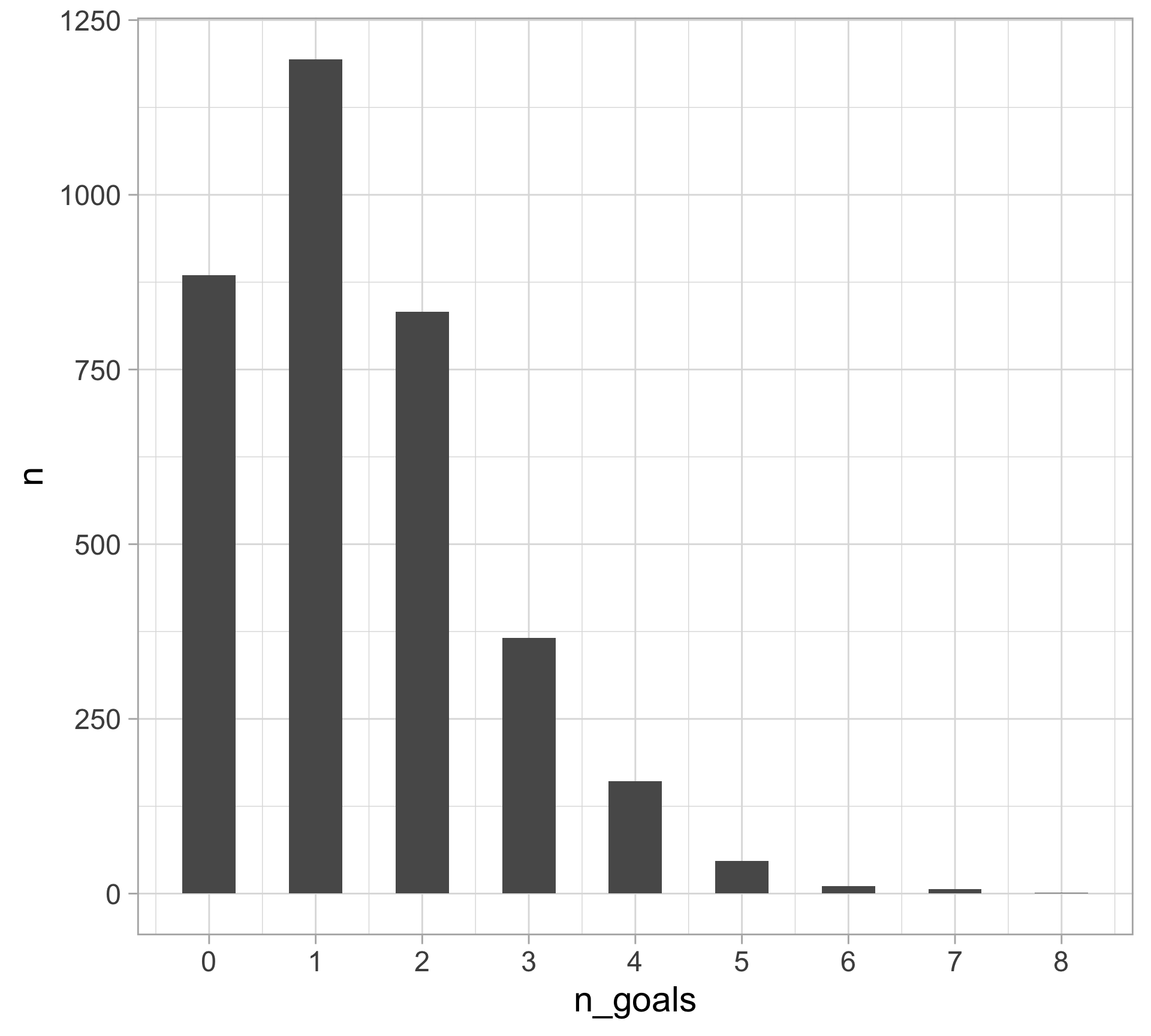
$ n_goals  <dbl> 1, 0, 1, 0, 1, 2, 1, 2, 0, 1, 1, 2, 1, 3, 1, 2, 2, 4, 1, 2, 0…
$ xG       <dbl> 2.4, 0.5, 0.3, 0.5, 1.3, 1.2, 2.3, 1.6, 1.0, 1.0, 0.5, 1.6, 0…
$ off_team <chr> "Manchester Utd", "Ipswich Town", "Newcastle Utd", "Everton",…
$ def_team <chr> "Fulham", "Liverpool", "Southampton", "Brighton", "Bournemout…
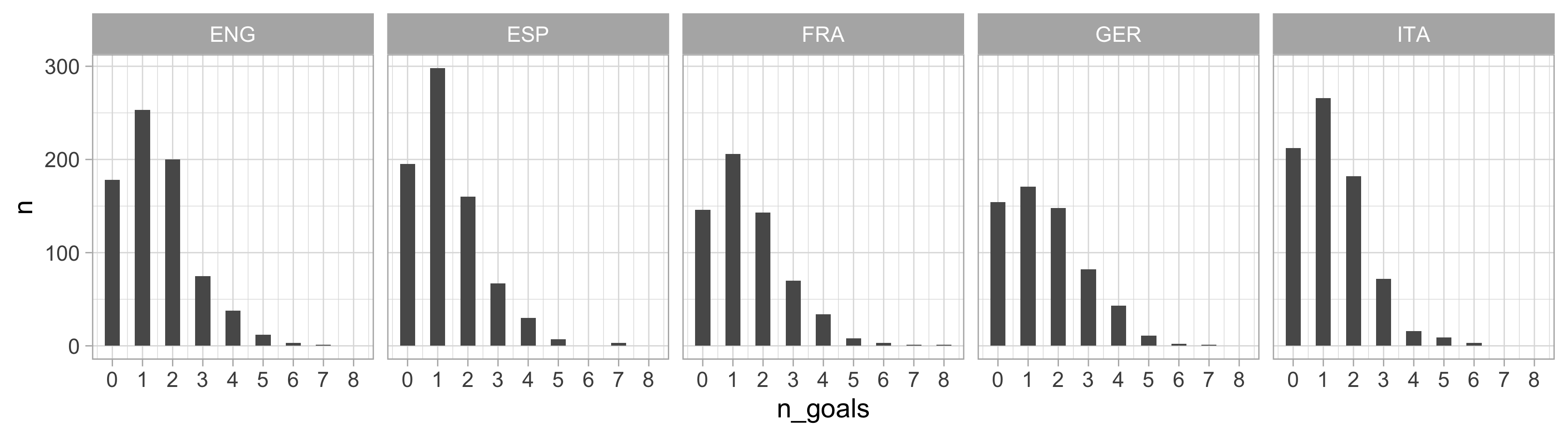
$ league   <chr> "ENG", "ENG", "ENG", "ENG", "ENG", "ENG", "ENG", "ENG", "ENG"…
$ match_id <dbl> 1, 2, 3, 4, 5, 6, 7, 8, 9, 10, 11, 12, 13, 14, 15, 16, 17, 18…
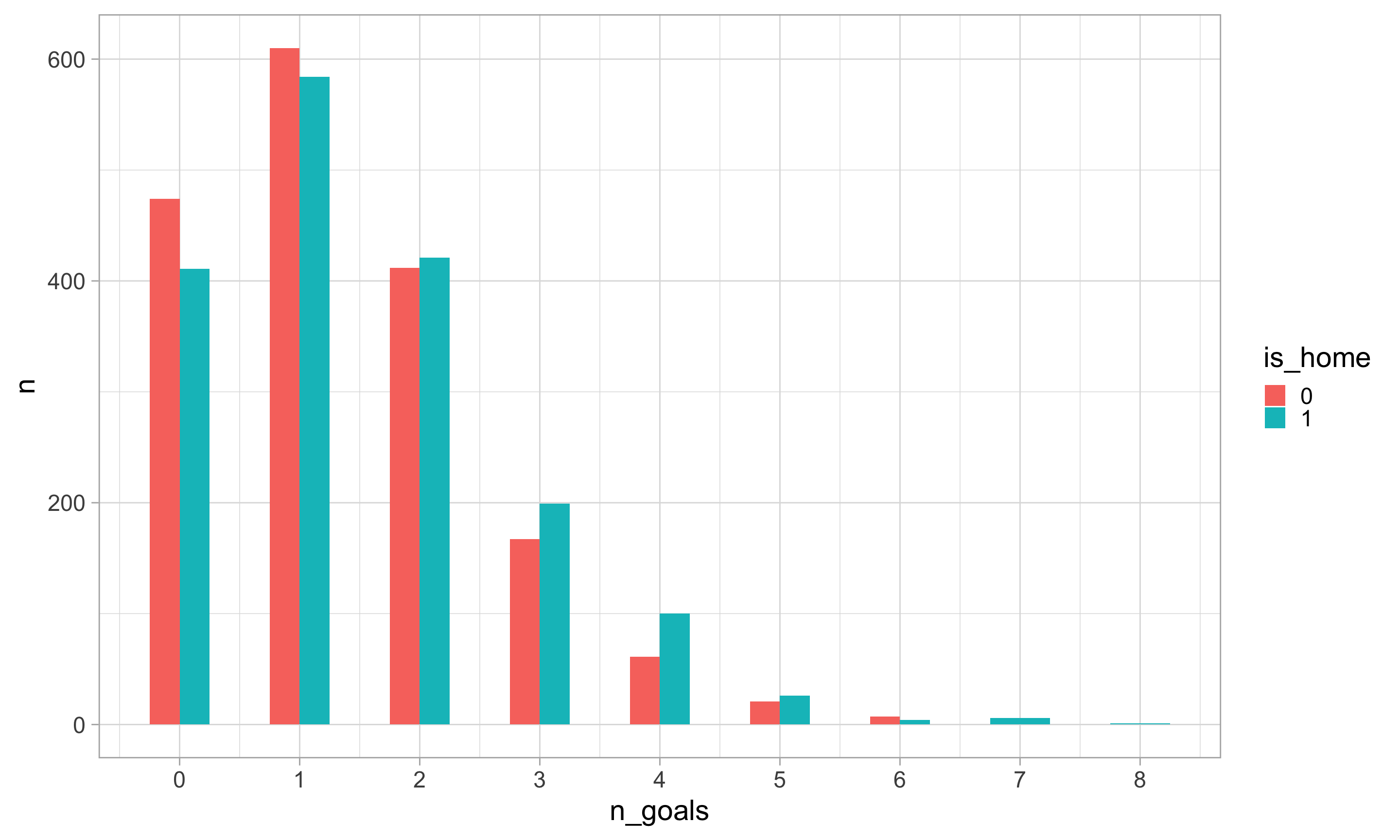
$ is_home  <dbl> 1, 1, 1, 1, 1, 1, 1, 1, 1, 1, 1, 1, 1, 1, 1, 1, 1, 1, 1, 1, 1…

EDA: Distribution for the number of goals

goals |> 
  count(n_goals) |> 
  ggplot(aes(n_goals, n)) +
  geom_col(width = 0.5) +
  scale_x_continuous(breaks = 0:8)

EDA: Distribution for the number of goals by league

goals |> 
  count(n_goals, league) |> 
  ggplot(aes(n_goals, n)) +
  geom_col(width = 0.5) +
  scale_x_continuous(breaks = 0:8) +
  facet_wrap(~ league, nrow = 1)

EDA: Distribution for the number of goals by home/away team

goals |> 
  count(n_goals, is_home) |> 
  mutate(is_home = factor(is_home)) |> 
  ggplot(aes(n_goals, n, fill = is_home, group = is_home)) +
  geom_col(position = "dodge", width = 0.5) +
  scale_x_continuous(breaks = 0:8)

Fitting a poisson regression model

goals_poisson <- glm(n_goals ~ league + is_home, family = "poisson", data = goals)
# summary(goals_poisson)
library(broom)
tidy(goals_poisson)
# A tibble: 6 × 5
  term        estimate std.error statistic  p.value
  <chr>          <dbl>     <dbl>     <dbl>    <dbl>
1 (Intercept)   0.321     0.0335     9.56  1.19e-21
2 leagueESP    -0.114     0.0436    -2.61  9.03e- 3
3 leagueFRA     0.0145    0.0447     0.325 7.45e- 1
4 leagueGER     0.0659    0.0440     1.50  1.35e- 1
5 leagueITA    -0.136     0.0439    -3.11  1.90e- 3
6 is_home       0.122     0.0285     4.27  1.92e- 5

What observations in the dataset correspond to predictions using only the intercept?

Fitting a poisson regression model

tidy(goals_poisson, exponentiate = TRUE, conf.int = TRUE)
# A tibble: 6 × 7
  term        estimate std.error statistic  p.value conf.low conf.high
  <chr>          <dbl>     <dbl>     <dbl>    <dbl>    <dbl>     <dbl>
1 (Intercept)    1.38     0.0335     9.56  1.19e-21    1.29      1.47 
2 leagueESP      0.892    0.0436    -2.61  9.03e- 3    0.819     0.972
3 leagueFRA      1.01     0.0447     0.325 7.45e- 1    0.929     1.11 
4 leagueGER      1.07     0.0440     1.50  1.35e- 1    0.980     1.16 
5 leagueITA      0.873    0.0439    -3.11  1.90e- 3    0.801     0.951
6 is_home        1.13     0.0285     4.27  1.92e- 5    1.07      1.19 

We have sufficient evidence to suggest the expected number of goals is different between ENG teams and each of ESP and ITA, but not FRA or GER, after accounting for home field advantage

The expected number of goals changes (is multiplied) by a factor of 1.13 (95% CI [1.07, 1.19]) if the team is home in comparison to away teams, after accounting for league

Model residuals and goodness-of-fit measures

  • Pearson residuals: \(\displaystyle r_i = \frac{y_i-\hat{\lambda}_i}{\sqrt{\hat{\lambda}_i}}\)

  • Deviance residuals: \(\displaystyle d_i = \textrm{sign}(y_i-\hat{\lambda}_i) \sqrt{2 \left[y_i \log\left(\frac{y_i}{\hat{\lambda}_i}\right) -(y_i - \hat{\lambda}_i) \right]}\)

residuals(goals_poisson, type = "pearson")
residuals(goals_poisson, type = "deviance")
  • Model summaries
glance(goals_poisson)
# A tibble: 1 × 8
  null.deviance df.null logLik    AIC    BIC deviance df.residual  nobs
          <dbl>   <int>  <dbl>  <dbl>  <dbl>    <dbl>       <int> <int>
1         4269.    3503 -5319. 10650. 10687.    4221.        3498  3504

As before, we prefer assessment in terms of out-of-sample/test set performances over these measures

Overdispersion

  • Overdispersion is a common problem faced in Poisson regression when the variance is larger than what is assumed under the model
  • Recall that a Poisson distribution assumes equidispersion (i.e. the mean and variance are equal)
  • Any concerns here?
var(goals$n_goals)
[1] 1.519783
mean(goals$n_goals)
[1] 1.413527

Negative binomial regression

Key idea: introduces another parameter such that the variance can exceed the mean

We have \(E(Y) = \lambda\) and \(\text{Var}(Y)=\lambda(1+\alpha \lambda)\)

  • The variance is still proportional to \(\lambda\), but depends on the dispersion parameter \(\alpha \ge 0\)
  • The further \(\alpha\) falls above 0, the greater the overdispersion relative to Poisson variability
  • As \(\alpha\) decreases toward 0, the variance decreases toward \(\lambda\) , and the model converges to a Poisson distribution

See here for more information

Negative binomial regression

goals_nb <- MASS::glm.nb(n_goals ~ league + is_home, data = goals)
summary(goals_nb)

Call:
MASS::glm.nb(formula = n_goals ~ league + is_home, data = goals, 
    init.theta = 23.79903563, link = log)

Coefficients:
            Estimate Std. Error z value Pr(>|z|)    
(Intercept)  0.32064    0.03453   9.286  < 2e-16 ***
leagueESP   -0.11413    0.04487  -2.544  0.01097 *  
leagueFRA    0.01435    0.04603   0.312  0.75530    
leagueGER    0.06584    0.04543   1.449  0.14726    
leagueITA   -0.13628    0.04512  -3.021  0.00252 ** 
is_home      0.12180    0.02931   4.156 3.24e-05 ***
---
Signif. codes:  0 '***' 0.001 '**' 0.01 '*' 0.05 '.' 0.1 ' ' 1

(Dispersion parameter for Negative Binomial(23.799) family taken to be 1)

    Null deviance: 4060.9  on 3503  degrees of freedom
Residual deviance: 4015.6  on 3498  degrees of freedom
AIC: 10646

Number of Fisher Scoring iterations: 1

              Theta:  23.8 
          Std. Err.:  10.2 

 2 x log-likelihood:  -10631.63 

Zero-inflated Poisson regression

  • One common problem in modeling count data is the prevalence of zeros
  • While the Poisson distribution allows for zero counts, there are problems with a lot more zeros observed than expected for Poisson data
  • A zero-inflated Poisson (ZIP) model is a mixture model with two components

    • Logistic regression model to predict whether the response will be zero (whether 0 goals are observed) \[P(Y = 0) = \pi + (1 - \pi)e^{\lambda}\]

    • Poisson regression model for non-zero counts (non-zero goal values) \[P(Y = y) = (1 - \pi) \frac{\lambda^y e^{-\lambda}}{y!}, \text{ for } y = 1, 2, 3, \dots\]

Zero-inflated Poisson (ZIP) regression

library(pscl) # install.packages("pscl")
goals_zip <- zeroinfl(n_goals ~ league + is_home, data = goals)
summary(goals_zip)

Call:
zeroinfl(formula = n_goals ~ league + is_home, data = goals)

Pearson residuals:
    Min      1Q  Median      3Q     Max 
-1.2381 -1.0887 -0.3100  0.5239  5.0085 

Count model coefficients (poisson with log link):
             Estimate Std. Error z value Pr(>|z|)    
(Intercept)  0.336872   0.039204   8.593  < 2e-16 ***
leagueESP   -0.141382   0.049638  -2.848  0.00440 ** 
leagueFRA    0.002821   0.057836   0.049  0.96110    
leagueGER    0.124432   0.059075   2.106  0.03517 *  
leagueITA   -0.152638   0.055749  -2.738  0.00618 ** 
is_home      0.142767   0.034039   4.194 2.74e-05 ***

Zero-inflation model coefficients (binomial with logit link):
            Estimate Std. Error z value Pr(>|z|)    
(Intercept)  -4.1160     0.9155  -4.496 6.92e-06 ***
leagueESP    -8.4725    48.4009  -0.175    0.861    
leagueFRA    -0.5554     2.0040  -0.277    0.782    
leagueGER     1.1872     1.0255   1.158    0.247    
leagueITA    -0.9125     2.5750  -0.354    0.723    
is_home       0.8414     0.8559   0.983    0.326    
---
Signif. codes:  0 '***' 0.001 '**' 0.01 '*' 0.05 '.' 0.1 ' ' 1 

Number of iterations in BFGS optimization: 52 
Log-likelihood: -5312 on 12 Df

Model comparison: Poisson vs ZIP

  • 5-fold cross-validation: assigning matches to folds (given the structure of the data—each match has 2 rows)
set.seed(2008)
N_FOLDS <- 5
goals_folds <- goals |> 
  distinct(match_id) |>
  mutate(match_fold = sample(rep(1:N_FOLDS, length.out = n())))

# goals_folds |> count(match_fold)

goals <- goals |> 
  left_join(goals_folds, by = "match_id")

Cross-validation

goals_cv <- function(x) {
  goals_train <- goals |> filter(match_fold != x)
  goals_test <- goals |> filter(match_fold == x)
  
  poisson_fit <- glm(n_goals ~ league + is_home, family = "poisson", data = goals_train)
  zip_fit <- zeroinfl(n_goals ~ league + is_home, data = goals_train)
  
  goals_out <- tibble(
    poisson_pred = predict(poisson_fit, newdata = goals_test, type = "response"),
    zip_pred = predict(zip_fit, newdata = goals_test),
    test_actual = goals_test$n_goals,
    test_fold = x
  )
  return(goals_out)  
}

goals_preds <- map(1:N_FOLDS, goals_cv) |> 
  bind_rows()

Out-of-sample comparison

Which model would you select?

goals_preds |> 
  pivot_longer(cols = poisson_pred:zip_pred, 
               names_to = "model", 
               values_to = "test_pred") |> 
  group_by(model, test_fold) |>
  summarize(rmse = sqrt(mean((test_actual - test_pred)^2))) |> 
  group_by(model) |> 
  summarize(cv_rmse = mean(rmse),
            se_rmse = sd(rmse) / sqrt(N_FOLDS))
# A tibble: 2 × 3
  model        cv_rmse se_rmse
  <chr>          <dbl>   <dbl>
1 poisson_pred    1.23  0.0107
2 zip_pred        1.23  0.0107

Remember: Occam’s razor

Resources

Appendix: Code to build dataset

library(worldfootballR)
library(tidyverse)
big5 <- fb_match_results(country = c("ENG", "ESP", "ITA", "GER", "FRA"),
                         gender = "M", 
                         season_end_year = 2025, 
                         tier = "1st")
big5 <- big5 |>
  mutate(match_id = row_number()) |>  # add unique id for each row
  filter(!is.na(Wk))
  
home_goals <- big5 |>
  select(n_goals = HomeGoals, xG = Home_xG, off_team = Home, def_team = Away, league = Country, match_id) |>
  mutate(is_home = 1)

away_goals <- big5 |>
  select(n_goals = AwayGoals, xG = Away_xG, off_team = Away, def_team = Home, league = Country, match_id) |>
  mutate(is_home = 0)

goals <- home_goals |>
  bind_rows(away_goals)
  
# write_csv(goals, "goals.csv")