Unsupervised learning: Gaussian mixture models

SURE 2025

Department of Statistics & Data Science
Carnegie Mellon University

Background

Previously: clustering

Goal: partition observations into subgroups/cluster, where points within a cluster are more “similar” than points between clusters

Classification vs clustering

Classification

Supervised learning
We are given labeled (categorical) data
Focus on generalizability (i.e. build a classifier that performs well on predicting unseen/test data)

Clustering

Unsupervised learning
We are only given the data points (with no labels)
Focus on finding interesting subgroups/structure in the data

Previously: clustering

Previous methods: \(k\)-means clustering and hierarchical clustering

Output hard assignments, strictly assigning observations to only one cluster

What about soft/fuzzy assignments and uncertainty in the clustering results?
- Assigns each observation a probability of belonging to a cluster
- Incorporate statistical modeling into clustering

We want to estimate the density of the observations in some way that allows us to extract clusters

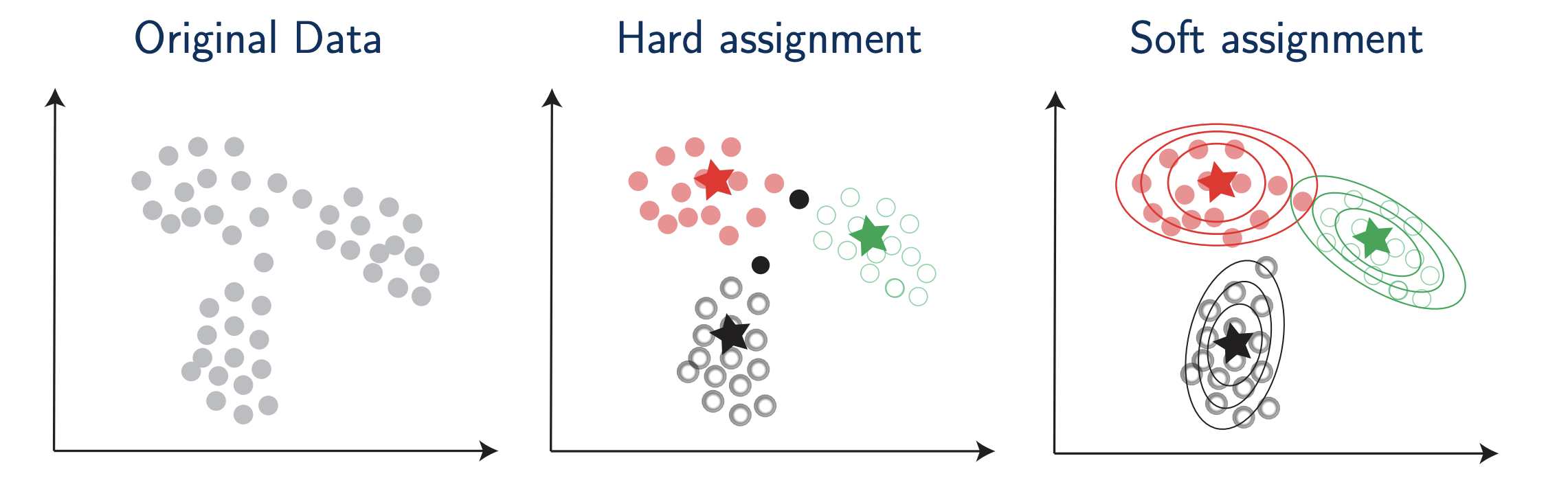
Motivating figure

Model-based (parametric) clustering

Moves beyond hard cluster assignments and allows for flexible and probabilistic soft assignments

Key idea: data are considered as coming from a mixture of underlying probability distributions

Assume data are sample from a population with underlying density; estimate density, use its characteristics to determine clustering structure

Most popular method: Gaussian mixture model (GMM)
- Each observation is assumed to be distributed as one of \(K\) multivariate normal distributions
- \(K\) is the number of clusters/components

Other variations: skewed normal, t-distributions, beta, etc. (as long as it can be estimated)

Mixture models

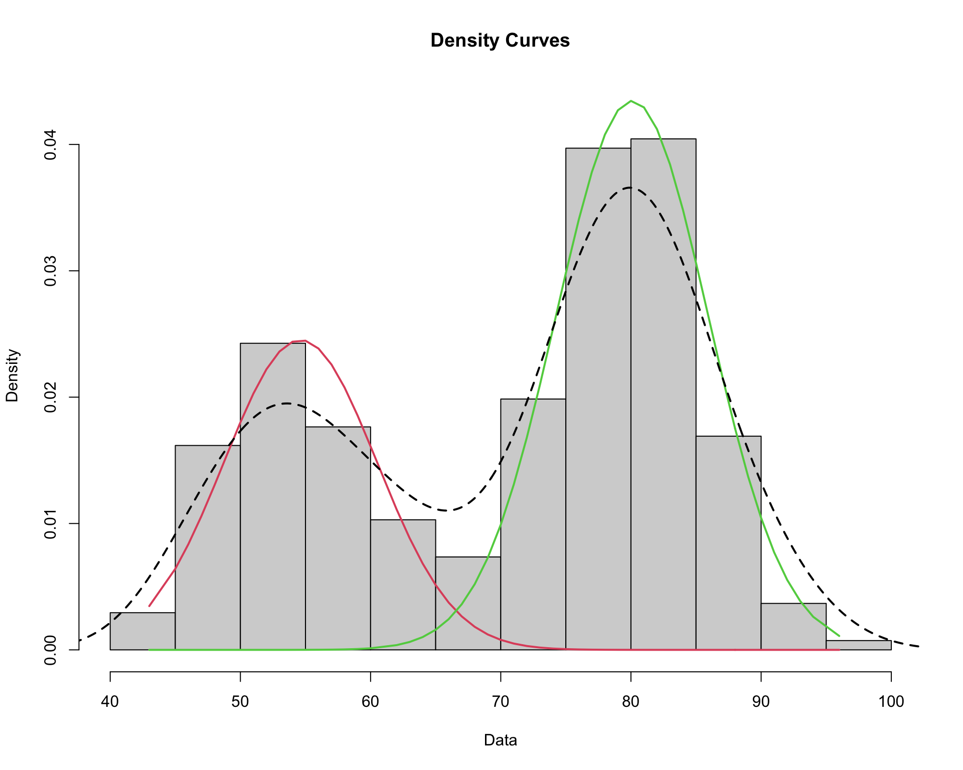
Mixtures of Gaussians in 1D

We would like to model the density of the data points, but due to the apparent multi-modality, a single Gaussian distribution would not be appropriate
There seems to be two separate underlying regimes, so instead we model the density as a mixture of Gaussians

number of iterations= 29

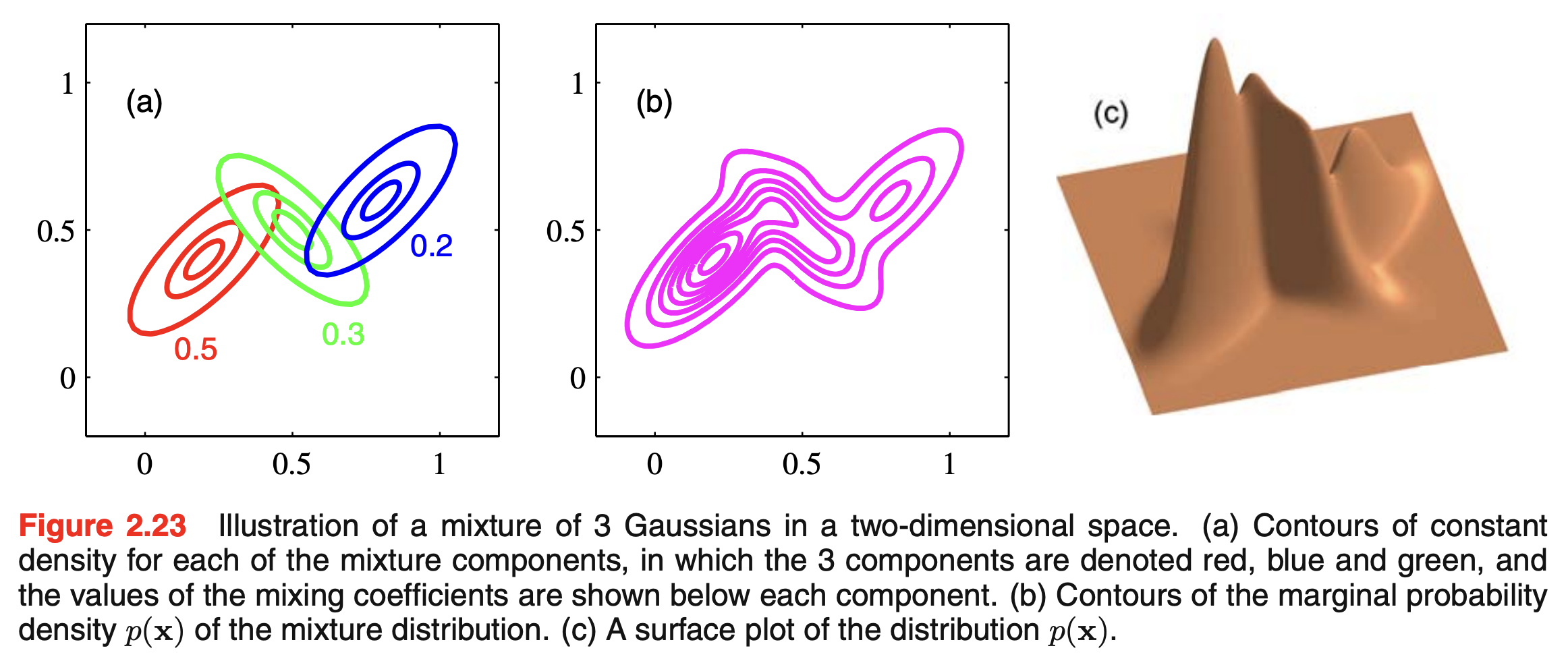
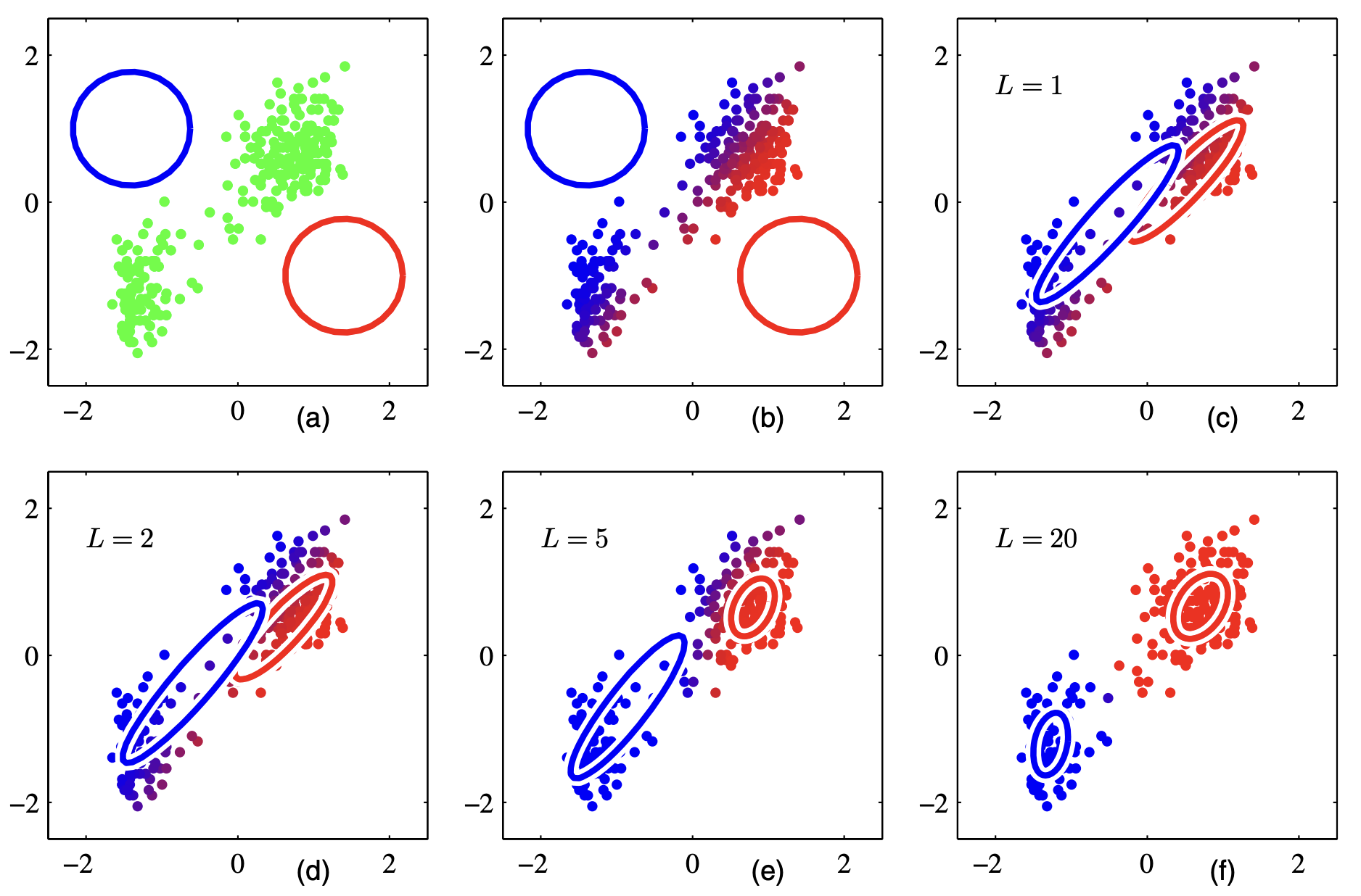
Mixtures of Gaussians in 2D

Mixture models in general

We assume that each population subgroup (cluster) is represented by some density \(f_k(x; \theta_k)\) and the population density \(f(x)\) is a weighted combination (i.e. mixture) of the subgroup densities

\[\displaystyle f(x) = \sum_{k=1}^K \tau_k f_k(x; \theta_k)\]

where

\(\tau_k\): mixture weights, with \(\tau_k \ge 0\) and \(\sum_{k=1}^K \tau_k = 1\)
\(f_k\): mixture components
\(K\): total number of mixture components (clusters)

We need to

choose the number of components (clusters) \(K\) and the weights \(\tau_k\)
estimate the parameters \(\theta_k\) of the mixture component densities \(f_k\)

Gaussian mixture models

Assume a parametric mixture model (with parameters \(\theta_k\) for the \(k\)-th component)

\[f(x) = \sum_{k=1}^K \tau_k f_k(x; \theta_k)\]

Most often the mixture component densities are assumed to be Gaussian with parameters \(\theta_k = \{\mu_k, \Sigma_k\}\)

The covariance matrices \(\Sigma_k\) characterize the clusters
- volume: size of the clusters (number of observations)
- shape: direction of variance (which variables display more variance)
- orientation: aligned with axes (low covariance) versus tilted (due to relationships between variables)

We can choose each of these values (volume/shape/orientation) to be the same or different among clusters

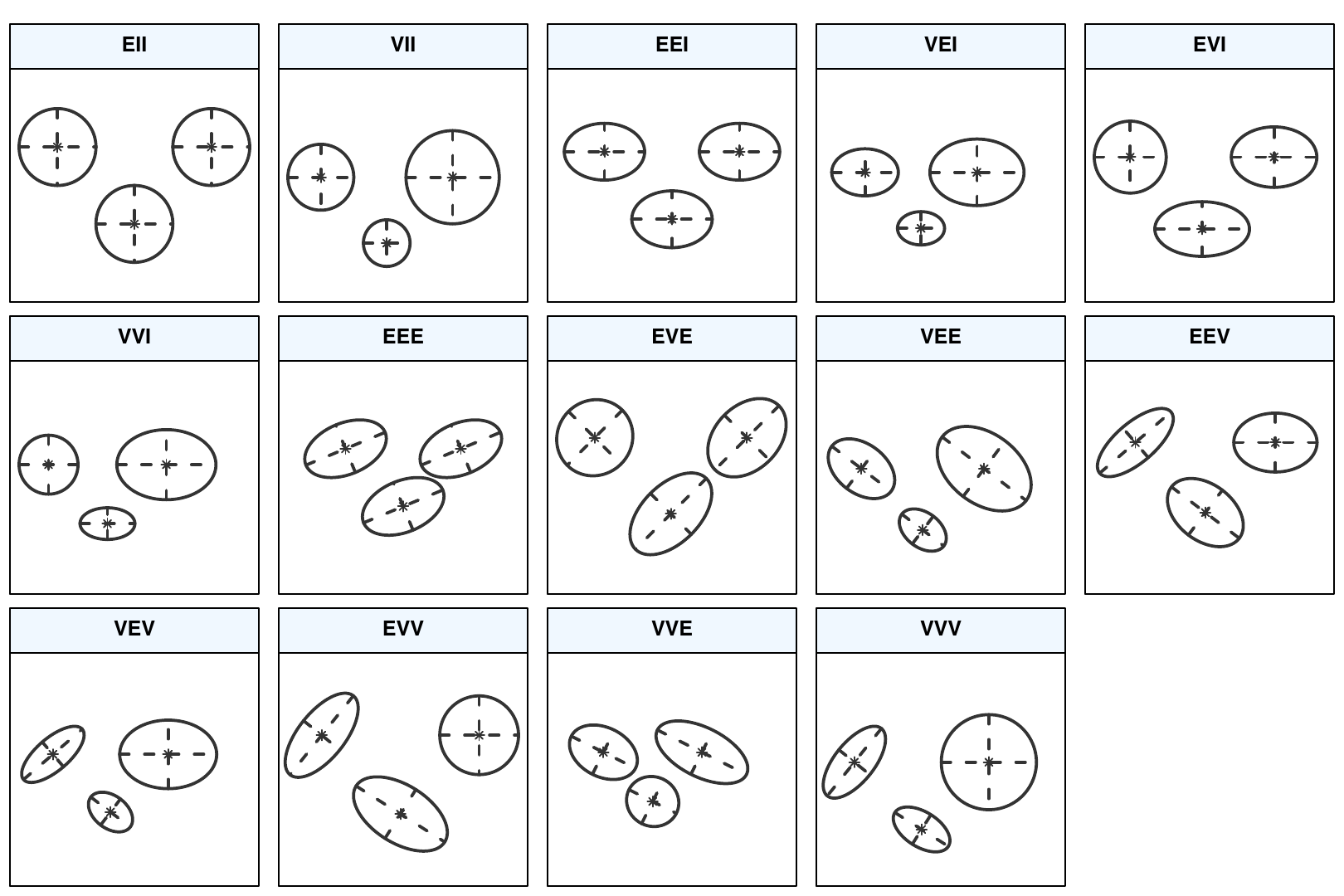
Covariance constraints

3 letters in model name denote (in order) the volume, shape, and orientation across clusters

Covariance constraints: summary table

Model	Distribution	Volume	Shape	Orientation
EII	Spherical	Equal	Equal	–
VII	Spherical	Variable	Equal	–
EEI	Diagonal	Equal	Equal	Coordinate axes
VEI	Diagonal	Variable	Equal	Coordinate axes
EVI	Diagonal	Equal	Variable	Coordinate axes
VVI	Diagonal	Variable	Variable	Coordinate axes
EEE	Ellipsoidal	Equal	Equal	Equal
EVE	Ellipsoidal	Equal	Variable	Equal
VEE	Ellipsoidal	Variable	Equal	Equal
VVE	Ellipsoidal	Variable	Variable	Equal
EEV	Ellipsoidal	Equal	Equal	Variable
VEV	Ellipsoidal	Variable	Equal	Variable
EVV	Ellipsoidal	Equal	Variable	Variable
VVV	Ellipsoidal	Variable	Variable	Variable

Model fitting and selection

Model fitting is done using an Expectation-Maximization (EM) algorithm

Since this is a statistical model, we can choose the number of components/clusters \(K\) and covariance constraint using the Bayesian Information Criterion (BIC) \[\text{BIC} = 2\log L(x \mid \theta) - m\log n \,,\] where
- \(L(x \mid \theta)\): likelihood of the considered model
- \(m\): number of parameters (e.g. VVV has the most parameters)
- \(n\): number of observations

The BICs are calculated for all candidate models (different combinations of \(K\) and covariance constraints), and we select one final model that gives the optimum BIC value

Expectation-Maximization (EM) algorithm

Goal: Given a GMM, we want to maximize the likelihood function with respect to the parameters (means & covariances of the components and mixture weights)

First, initialize the model parameters (\(\mu_k, \Sigma_k, \tau_k\)) randomly

Then, alternate between the following two steps (keep repeating until convergence)
- E-step: estimate \(\gamma_{ik}\), the soft assignments of observation \(i\) belonging to component/cluster \(k\)
- M-step: re-estimate the model parameters

Output: \(\hat{\gamma}_{ik}\) are the final estimated soft assignments of observation \(i\) belonging to cluster \(k\)
- We can assign observation \(i\) to a cluster with the largest \(\hat{\gamma}_{ik}\)
- We also get the cluster assignment uncertainty of \(\displaystyle 1 - \max_k \hat{\gamma}_{ik}\)

EM algorithm example

Is this familiar?

In GMMs, we’re essentially
- guessing how much we think each Gaussian component generates each observation
- pretending to know the parameters to perform maximum likelihood estimation

This resembles the \(k\)-means algorithm!
- The cluster centroids are chosen at random, and then recomputed/updated
- This is repeated until the cluster assignments stop changing

Instead of assigning each point to a single cluster, we “softly” assign them so they contribute fractionally to each cluster

Example

Data: NBA player statistics per 100 possessions (2023-24 regular season)

library(tidyverse)
theme_set(theme_light())
nba_players <- read_csv("https://raw.githubusercontent.com/36-SURE/2025/main/data/nba_players_2024.csv")
glimpse(nba_players)

Rows: 452
Columns: 33
$ rk         <dbl> 1, 2, 3, 4, 5, 6, 7, 9, 10, 11, 12, 13, 14, 16, 17, 19, 20,…
$ player     <chr> "Precious Achiuwa", "Bam Adebayo", "Ochai Agbaji", "Santi A…
$ pos        <chr> "PF-C", "C", "SG", "PF", "SG", "SG", "C", "PG", "PF", "PF",…
$ age        <dbl> 24, 26, 23, 23, 25, 28, 25, 25, 30, 29, 31, 23, 26, 23, 25,…
$ tm         <chr> "TOT", "MIA", "TOT", "MEM", "MIN", "PHO", "CLE", "NOP", "MI…
$ g          <dbl> 74, 71, 78, 61, 82, 75, 77, 56, 79, 73, 34, 81, 50, 75, 55,…
$ gs         <dbl> 18, 71, 28, 35, 20, 74, 77, 0, 10, 73, 0, 0, 50, 75, 55, 1,…
$ mp         <dbl> 1624, 2416, 1641, 1618, 1921, 2513, 2442, 1028, 1782, 2567,…
$ fg         <dbl> 7.2, 10.9, 5.2, 7.5, 6.1, 6.6, 10.5, 6.8, 5.5, 15.7, 5.0, 9…
$ fga        <dbl> 14.4, 21.0, 12.7, 17.2, 13.8, 13.3, 16.6, 16.5, 12.0, 25.6,…
$ fgpercent  <dbl> 0.501, 0.521, 0.411, 0.435, 0.439, 0.499, 0.634, 0.412, 0.4…
$ x3p        <dbl> 0.8, 0.3, 1.8, 3.2, 3.4, 4.0, 0.0, 3.7, 0.3, 0.6, 0.0, 2.5,…
$ x3pa       <dbl> 3.0, 0.9, 6.2, 9.2, 8.6, 8.6, 0.1, 9.9, 1.3, 2.3, 0.3, 7.5,…
$ x3ppercent <dbl> 0.268, 0.357, 0.294, 0.349, 0.391, 0.461, 0.000, 0.377, 0.2…
$ x2p        <dbl> 6.4, 10.6, 3.4, 4.3, 2.7, 2.6, 10.5, 3.1, 5.2, 15.0, 5.0, 6…
$ x2pa       <dbl> 11.4, 20.1, 6.5, 8.0, 5.2, 4.6, 16.4, 6.6, 10.7, 23.3, 9.0,…
$ x2ppercent <dbl> 0.562, 0.528, 0.523, 0.534, 0.517, 0.570, 0.638, 0.464, 0.4…
$ ft         <dbl> 2.1, 6.0, 1.1, 1.6, 1.3, 2.5, 4.7, 1.7, 2.7, 9.6, 0.0, 4.9,…
$ fta        <dbl> 3.4, 8.0, 1.6, 2.6, 1.7, 2.9, 6.4, 2.5, 3.8, 14.6, 0.6, 5.9…
$ ftpercent  <dbl> 0.616, 0.755, 0.661, 0.621, 0.800, 0.878, 0.742, 0.673, 0.7…
$ orb        <dbl> 5.9, 3.3, 2.2, 2.2, 0.9, 0.9, 4.9, 1.2, 1.7, 3.7, 2.2, 1.7,…
$ drb        <dbl> 9.1, 11.9, 4.2, 8.5, 3.4, 4.8, 11.5, 4.9, 5.9, 12.1, 1.9, 6…
$ trb        <dbl> 14.9, 15.2, 6.4, 10.6, 4.3, 5.7, 16.4, 6.1, 7.6, 15.7, 4.0,…
$ ast        <dbl> 3.0, 5.7, 2.4, 4.2, 5.2, 4.4, 4.2, 5.6, 9.2, 8.9, 5.3, 6.4,…
$ stl        <dbl> 1.4, 1.7, 1.4, 1.3, 1.6, 1.3, 1.1, 2.8, 2.0, 1.6, 2.2, 1.7,…
$ blk        <dbl> 2.1, 1.4, 1.3, 1.6, 1.1, 0.9, 1.6, 0.7, 1.3, 1.5, 1.2, 1.0,…
$ tov        <dbl> 2.5, 3.3, 1.9, 2.1, 2.0, 1.8, 2.4, 1.9, 2.5, 4.7, 4.3, 3.4,…
$ pf         <dbl> 4.4, 3.3, 3.4, 2.7, 3.7, 3.1, 3.0, 4.2, 3.6, 3.9, 7.4, 4.8,…
$ pts        <dbl> 17.3, 28.2, 13.4, 19.8, 16.9, 19.7, 25.7, 18.9, 14.0, 41.6,…
$ x          <lgl> NA, NA, NA, NA, NA, NA, NA, NA, NA, NA, NA, NA, NA, NA, NA,…
$ ortg       <dbl> 114, 115, 102, 109, 115, 130, 131, 112, 114, 126, 92, 110, …
$ drtg       <dbl> 112, 109, 121, 114, 111, 117, 110, 112, 109, 112, 117, 111,…
$ link       <chr> "/players/a/achiupr01.html", "/players/a/adebaba01.html", "…

Implementation with `mclust` package

Select the model and number of clusters

Use Mclust() function to search over 1 to 9 clusters (default) and the different covariance constraints (i.e. models)

library(mclust)
# x3pa: 3pt attempts per 100 possessions
# trb: total rebounds per 100 possessions
nba_mclust <- nba_players |> 
  select(x3pa, trb) |> 
  Mclust()
summary(nba_mclust)

---------------------------------------------------- 
Gaussian finite mixture model fitted by EM algorithm 
---------------------------------------------------- 

Mclust VVV (ellipsoidal, varying volume, shape, and orientation) model with 3
components: 

 log-likelihood   n df      BIC       ICL
      -2246.359 452 17 -4596.65 -4739.919

Clustering table:
  1   2   3 
 40 280 132

View clustering summary

library(broom)
nba_mclust |> 
  tidy()

# A tibble: 3 × 5
  component  size proportion mean.x3pa mean.trb
      <int> <int>      <dbl>     <dbl>    <dbl>
1         1    40     0.0822     0.101    15.5 
2         2   280     0.535      8.12      6.38
3         3   132     0.382      6.04     11.0

View clustering assignments

nba_mclust |> 
  augment() |> 
  ggplot(aes(x = x3pa, y = trb, color = .class, size = .uncertainty)) +
  geom_point(alpha = 0.6) +
  ggthemes::scale_color_colorblind()

Display the BIC for each model and number of clusters

nba_mclust |> 
  plot(what = "BIC", 
       legendArgs = list(x = "bottomright", ncol = 4))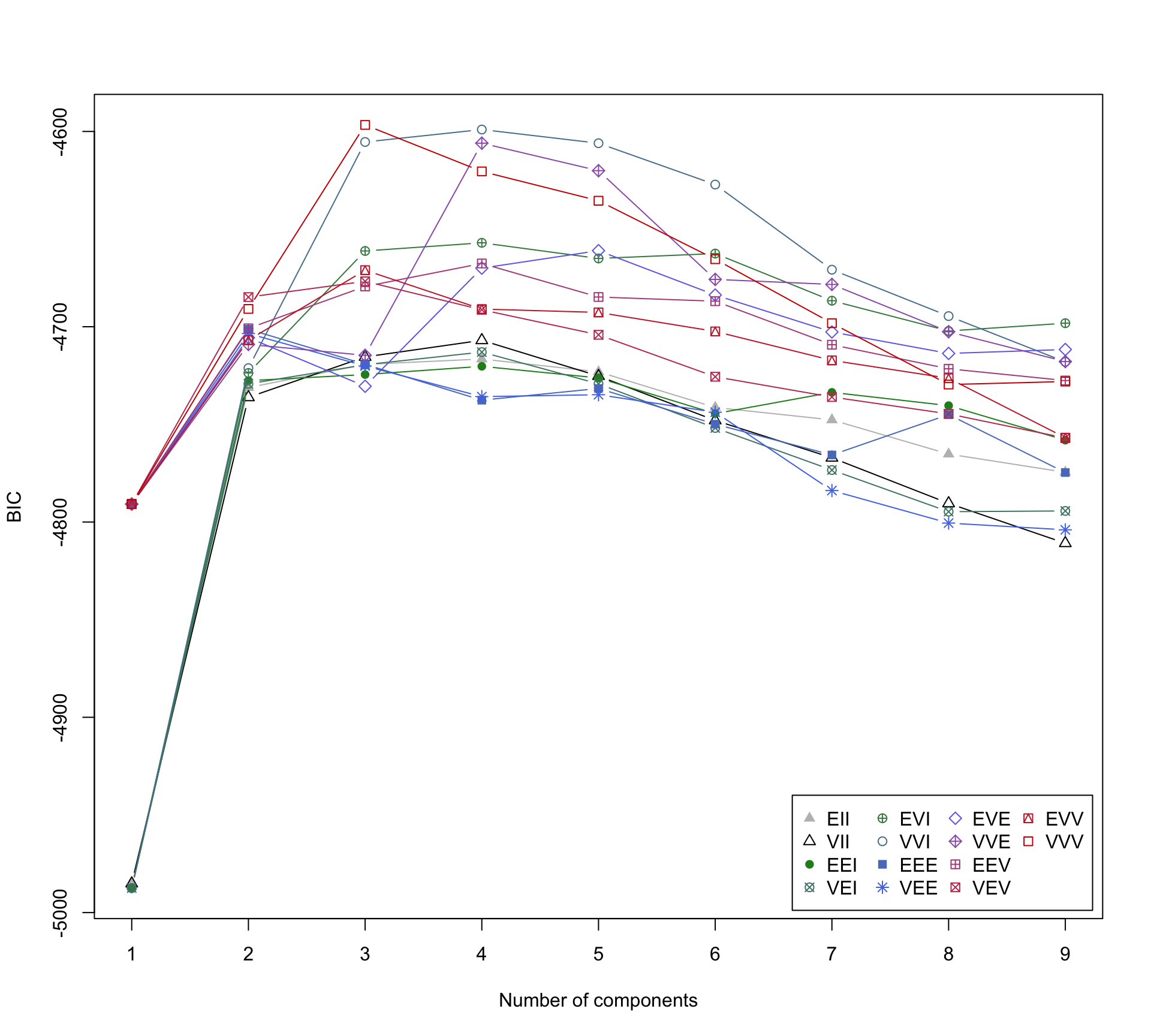

nba_mclust |> 
  plot(what = "classification")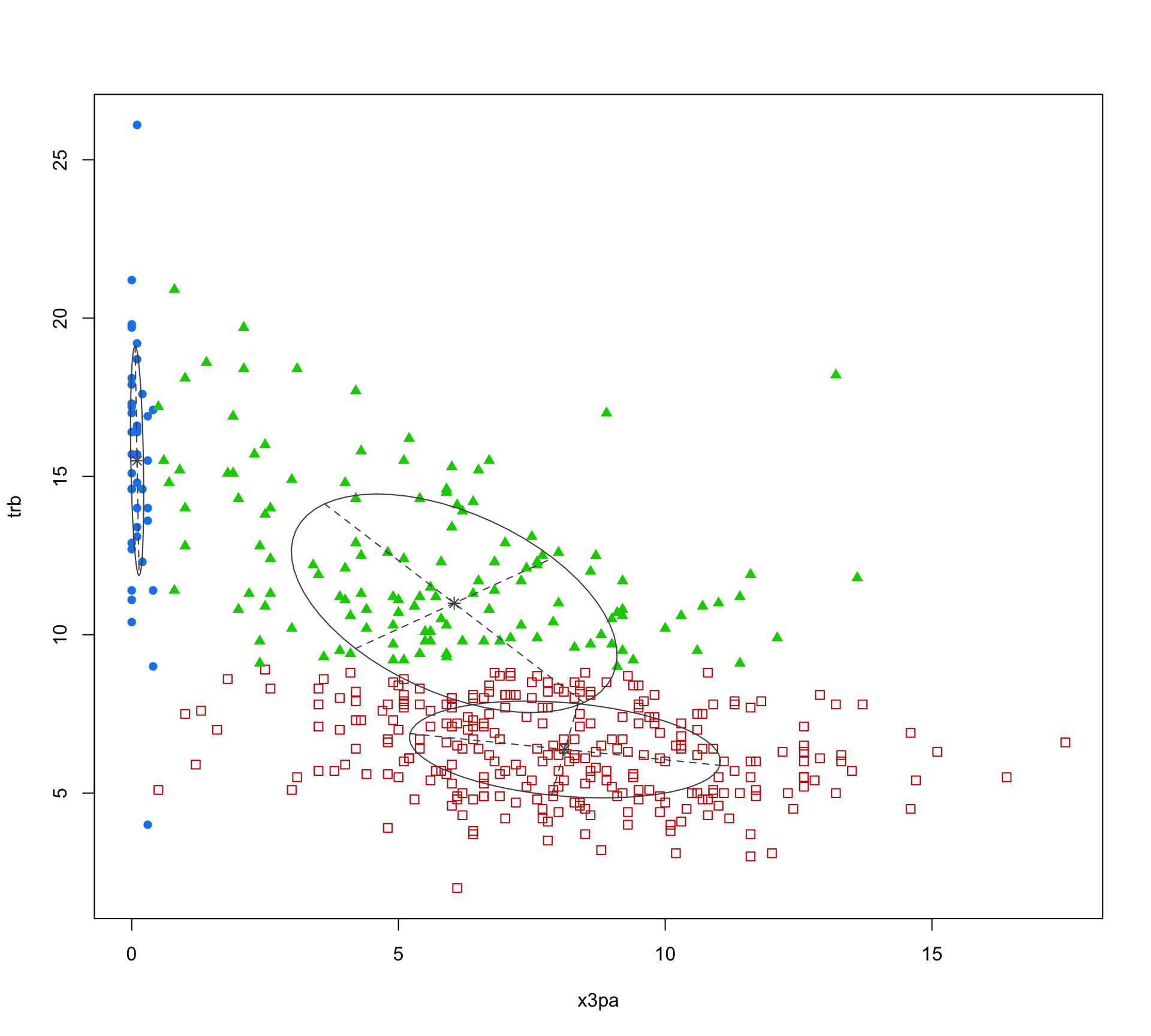

How do the cluster assignments compare to the positions?

Two-way table to compare the clustering assignments with player positions

(What’s the way to visually compare the two labels?)

table("Clusters" = nba_mclust$classification, "Positions" = nba_players$pos)

        Positions
Clusters  C C-PF PF PF-C PF-SF PG PG-SG SF SF-PF SF-SG SG SG-PG
       1 34    2  3    0     0  1     0  0     0     0  0     0
       2  3    0 33    0     1 78     4 70     1     1 88     1
       3 43    1 53    1     0  3     0 22     1     0  8     0

Takeaway: positions tend to fall within particular clusters

What about the cluster probabilities?

nba_player_probs <- nba_mclust$z
colnames(nba_player_probs) <- str_c("cluster", 1:3)

nba_player_probs <- nba_player_probs |>
  as_tibble() |>
  mutate(player = nba_players$player) |>
  pivot_longer(!player, names_to = "cluster", values_to = "prob")

nba_player_probs |>
  ggplot(aes(prob)) +
  geom_histogram() +
  facet_wrap(~ cluster)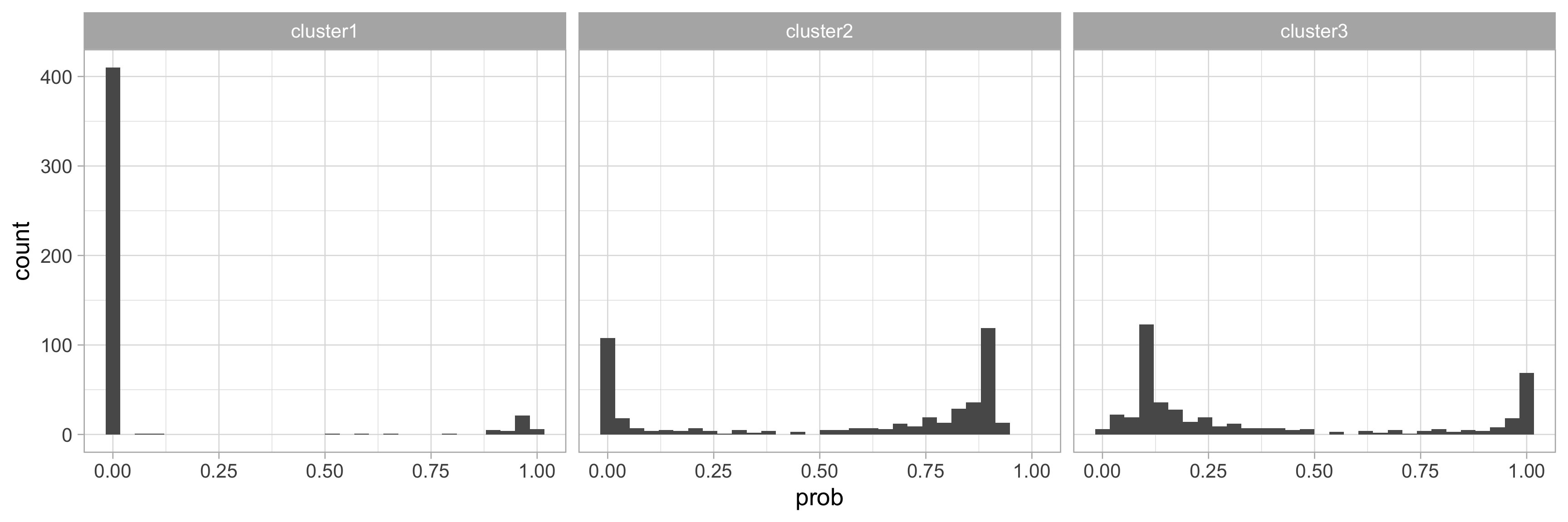

Which players have the highest uncertainty?

nba_players |>
  mutate(cluster = nba_mclust$classification,
         uncertainty = nba_mclust$uncertainty) |> 
  group_by(cluster) |>
  slice_max(uncertainty, n = 5) |> 
  mutate(player = fct_reorder(player, uncertainty)) |> 
  ggplot(aes(x = uncertainty, y = player)) +
  geom_point(size = 3) +
  facet_wrap(~ cluster, scales = "free_y", nrow = 3)

Challenges and resources

What if the data are not normal (ish) and instead are skewed?
- Apply a transformation, then perform GMM
- GMM on principal components of data
- Multivariate \(t\) mixture model
Review paper: Model-Based Clustering
Book: Model-Based Clustering and Classification for Data Science
Adrian Raftery’s website

Unsupervised learning: Gaussian mixture models

Background

Previously: clustering

Previously: clustering

Motivating figure

Model-based (parametric) clustering

Mixture models

Mixtures of Gaussians in 1D

Mixtures of Gaussians in 2D

Mixture models in general

Gaussian mixture models

Covariance constraints

Covariance constraints: summary table

Model fitting and selection

Expectation-Maximization (EM) algorithm

EM algorithm example

Is this familiar?

Example

Data: NBA player statistics per 100 possessions (2023-24 regular season)

Implementation with mclust package

View clustering summary

View clustering assignments

Display the BIC for each model and number of clusters

How do the cluster assignments compare to the positions?

What about the cluster probabilities?

Which players have the highest uncertainty?

Challenges and resources

Implementation with `mclust` package