Supervised learning: nonparametric regression

SURE 2025

Department of Statistics & Data Science
Carnegie Mellon University

Background

Recall: Model flexibility vs interpretability

• Generally speaking: trade-off between a model’s flexibility (i.e. how “wiggly” it is) and how interpretable it is

• Parametric methods (e.g. linear regression, GLMs): we make an assumption about the functional form, or shape, of \(f\) before observing the data

• Nonparametric methods: we do not make explicit assumptions about the functional form of \(f\) (i.e., \(f\) is estimated from the data)

• Parametric models are generally easier to interpret, whereas nonparametric models are more flexible

\(k\)-nearest neighbors (\(k\)-NN)

• Perhaps the simplest nonparametric method…

• Find the \(k\) data points closest to an observation \(x\), use these to make predictions

  • Need to use some measure of distance, e.g., Euclidean distance

• Take the average value of the response over the \(k\) nearest neighbors

  • \(k\)-NN classification: most common class among the \(k\) nearest neighbors (“majority vote”)

  • \(k\)-NN regression: average of the values of \(k\) nearest neighbors

• The number of neighbors \(k\) is a tuning parameter (like \(\lambda\) is for ridge/lasso)

Finding the optimal number of neighbors \(k\)

Recall: bias-variance tradeoff

• If \(k\) is too small, the resulting model is too flexible: low bias, high variance

• If \(k\) is too large, the resulting model is not flexible enough: high bias, low variance

Moving beyond linearity

• The truth is (almost) never linear

• But often the linearity assumption is good enough

• What if it’s not linear?

  • splines

  • local regression

  • generalized additive models

  • wavelets

• The above methods can offer a lot of flexibility, without losing the ease and interpretability of linear models

Generalized additive models (GAMs)

Resources

• Book: Generalized Additive Models by Simon Wood

• GAM resources GitHub repository

• mgcv workshop

• Free GAM Course

• Chapters 7 and 8

Generalized additive models (GAMs)

• Previously: generalized linear models (GLMs) (e.g., linear regression, logistic regression, Poisson regression)

• GLM generalizes linear regression to permit non-normal distributions and link functions of the mean \[g(\mathbb E[Y \mid X = x]) = \beta_0 + \beta_1 x_1 + \beta_2 x_2 + \dots + \beta_p x_p\]

• What if we replace the linear predictor by additive smooth functions of the explanatory variables?

• Entering generalized additive models (GAMs)

  • relax the restriction that the relationship must be a simple weighted sum

  • instead assume that the response can be modeled by a sum of arbitrary functions of each predictor

Generalized additive models (GAMs)

• Allows for flexible nonlinearities in several variables

• But retains the additive structure of linear models

\[g(\mathbb E[Y \mid X = x]) = \beta_0 + s_1(x_1) + s_2(x_2) + \dots + s_p(x_p)\]

• Like GLMs, a GAM specifies a link function \(g()\) and a probability distribution for the response \(Y\)

• \(s_j\) is some smooth function of predictor \(j\)

• GLM is the special case of GAM in which each \(s_j\) is a linear function

Why use smooth functions rather that just coefficients?

• Relationships between individual predictors and the response are smooth

• Estimate the smooth relationships simultaneously to predict the response by adding them up

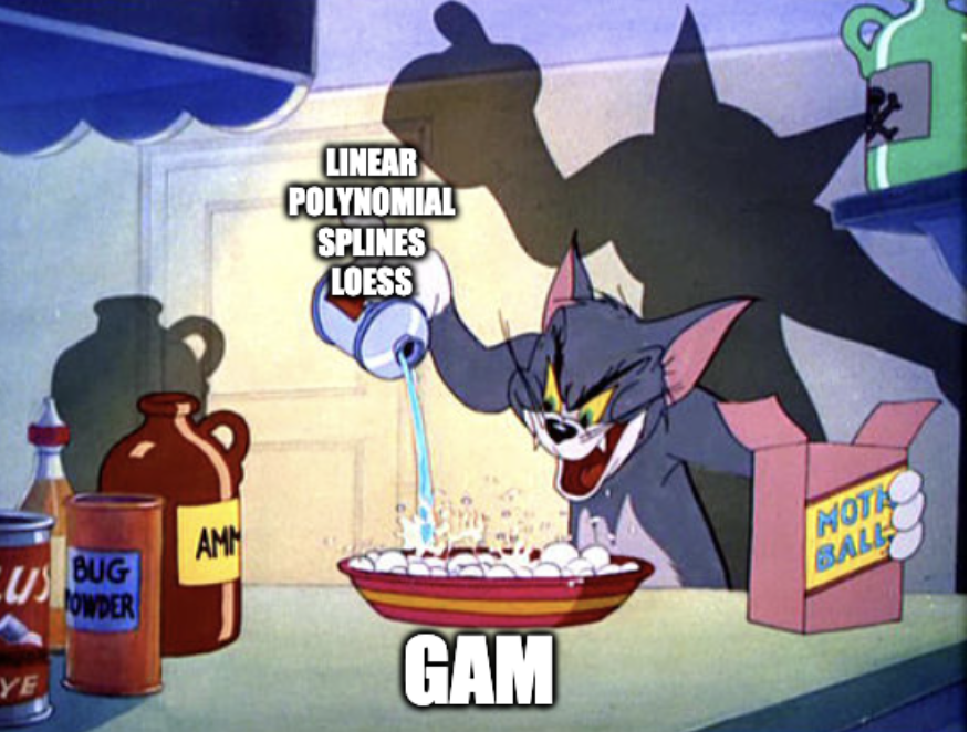
• GAMs have the advantage over GLMs of greater flexibility (want to model the covariates flexibly, covariates and response not necessarily linearly related)

• A disadvantage of GAMs/smoothing methods is the loss of interpretability

  • How do we interpret the effect of a predictor on the response?

  • How do we perform inferences for those effects?

Generalized additive models (GAMs)

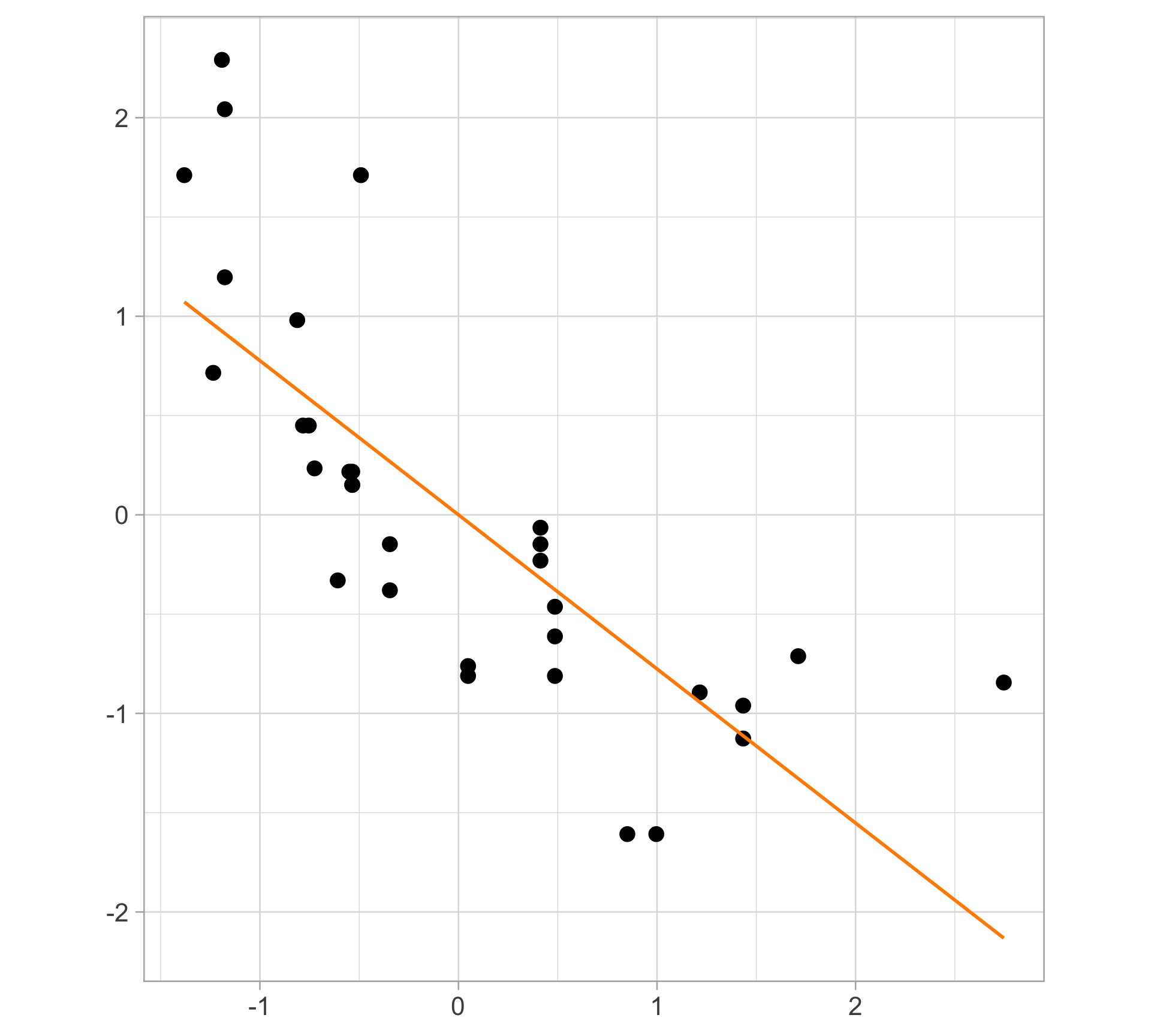
Toy example: is this linear?

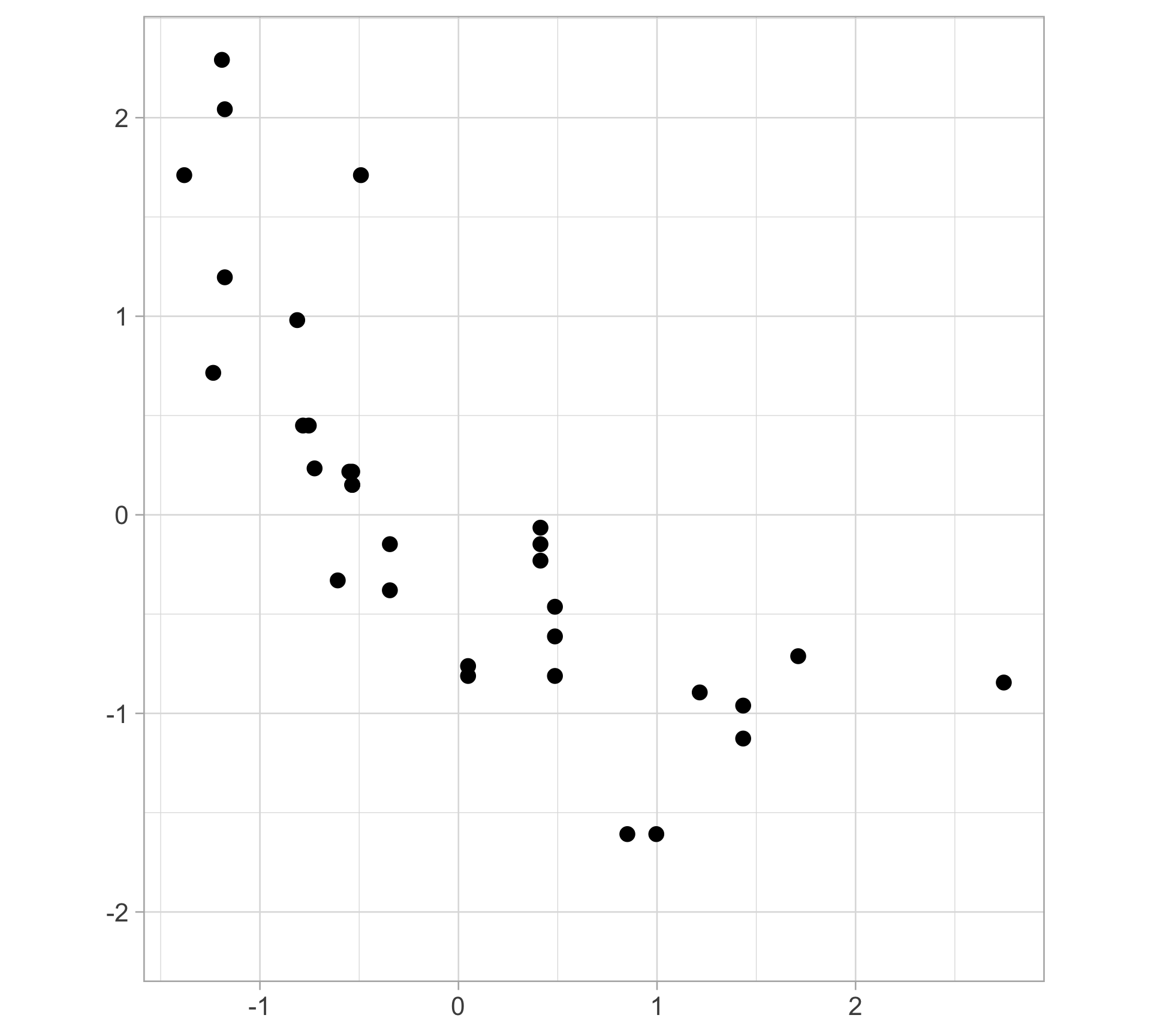
Toy example: linear regression fit

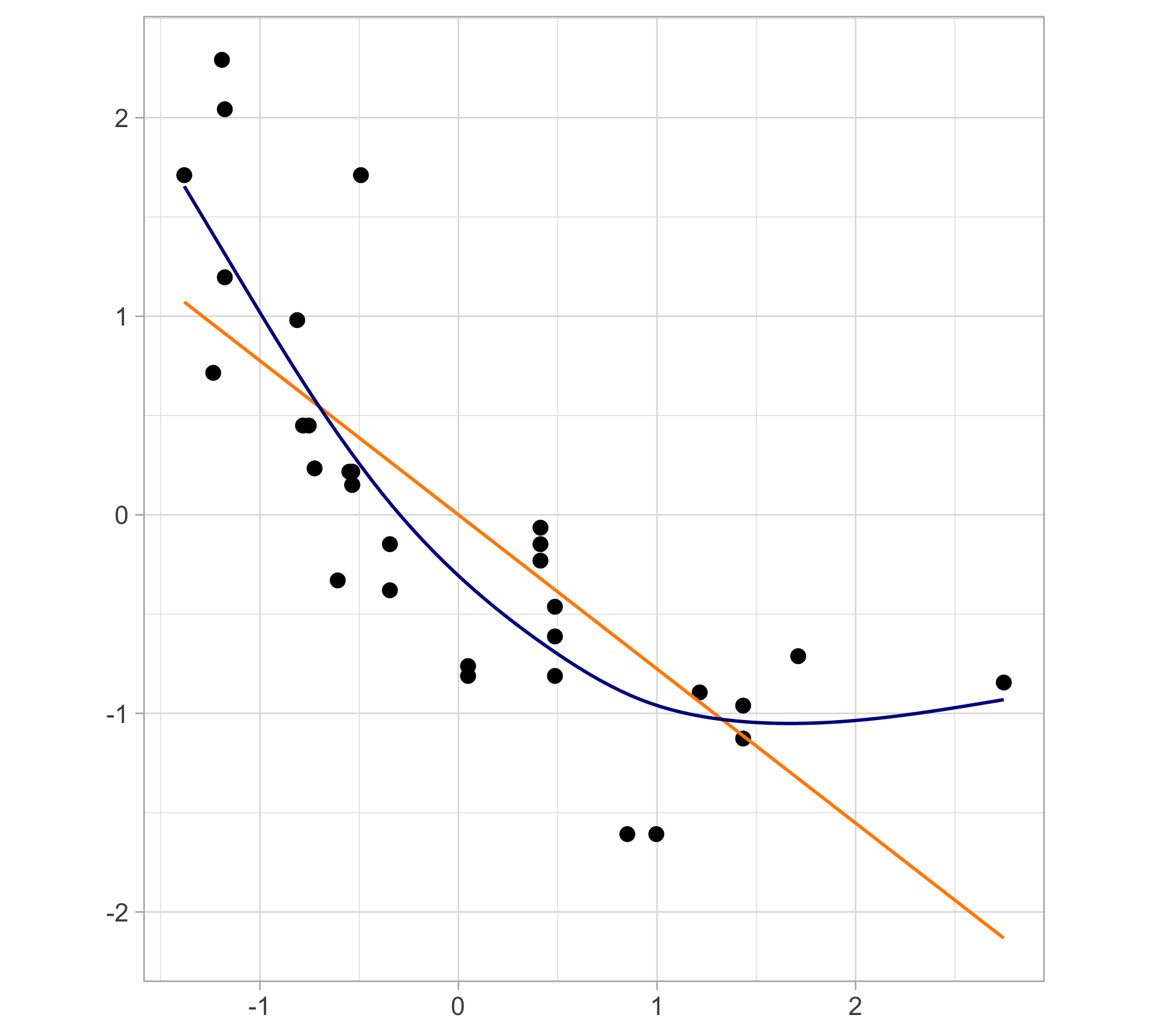
Toy example: GAM fit

Splines

• A common way to smooth and learn nonlinear functions is to use splines

• Splines can be used to approximate other, more complex functions

• Splines are functions that are constructed from simpler basis functions (usually polynomials), and the set of basis functions is a basis

• Each basis function \(b_k\) has coefficient \(\beta_k\). Spline is just the sum of the weighted basis functions

\[\displaystyle s(x) = \sum_{k=1}^K \beta_k b_k(x)\]

Weight basis functions to obtain spline

Why not just a polynomial fit?

\[y_i \sim \mathcal{N}(\mu_i, \sigma^2)\] \[\mu_i = \beta_0 + \beta_1 x_{i} + \beta_2 x^2_{1i} + \cdots + \beta_j x^j_{i}\]

• In the polynomial models we use a polynomial basis expansion of \(x\)

  • \(x^0 = 1\) (constant term), \(x, x^2, x^3, x^4, \dots\)

• We can keep on adding ever more powers of \(x\) to the model (hmm…)

• Runge phenomenon: oscillations at the edges of an interval—using higher-order polynomials doesn’t always improve accuracy

Smoothing splines

Use smooth function \(s(x)\) to predict \(y\), control smoothness directly by minimizing the spline objective function

\[\sum_{i=1}^n (y_i - s(x_i))^2 + \lambda \int s''(x)^2dx\]

\[= \text{fit data} + \text{impose smoothness}\]

\[\longrightarrow \text{model fit} = \text{likelihood} - \lambda \cdot \text{wiggliness}\]

Smoothing splines

• The most commonly considered case: cubic smoothing splines

\[\text{minimize }\sum_{i=1}^n (y_i - s(x_i))^2 + \lambda \int s''(x)^2dx\]

• First term: RSS, tries to make \(s(x)\) fit the data at each \(x_i\)

• Second term: roughness penalty, controls how wiggly \(s(x)\) is via tuning parameter \(\lambda \ge 0\)

  • Balances the accuracy of the fit and the flexibility of the function

  • The smaller \(\lambda\), the more wiggly the function

  • As \(\lambda \rightarrow \infty\), \(s(x)\) becomes linear

Smoothing splines

Goal: Estimate the smoothing spline \(\hat{s}(x)\) that balances the tradeoff between the model fit and wiggliness

Remember: Goldilocks principle

GAM recap

• A framework to model flexible nonlinear relationships

• Use little functions (basis functions) to make big functions (smooths)

• The predictor matrix has columns for each basis function, evaluated at each observation

• Use a penalty to trade off model fit and wiggliness

• Need to make sure the smooths are wiggly enough

Examples

Predicting MLB HR probability

• Data available via the pybaseball library in python

• Statcast data include pitch-level information, pulled from baseballsavant.com

• Example data collected for the entire month of May 2024

library(tidyverse)
savant <- read_csv("https://raw.githubusercontent.com/36-SURE/2025/main/data/savant.csv")
batted_balls <- savant |> 
  filter(type == "X") |> 
  mutate(is_hr = as.numeric(events == "home_run")) |> 
  filter(!is.na(launch_angle), !is.na(launch_speed), !is.na(is_hr))
# glimpse(batted_balls)

Predicting HRs with launch angle and exit velocity

HRs are relatively rare and confined to one area of this plot

batted_balls |> 
  ggplot(aes(x = launch_speed, 
             y = launch_angle, 
             color = as.factor(is_hr))) +
  geom_point(alpha = 0.2)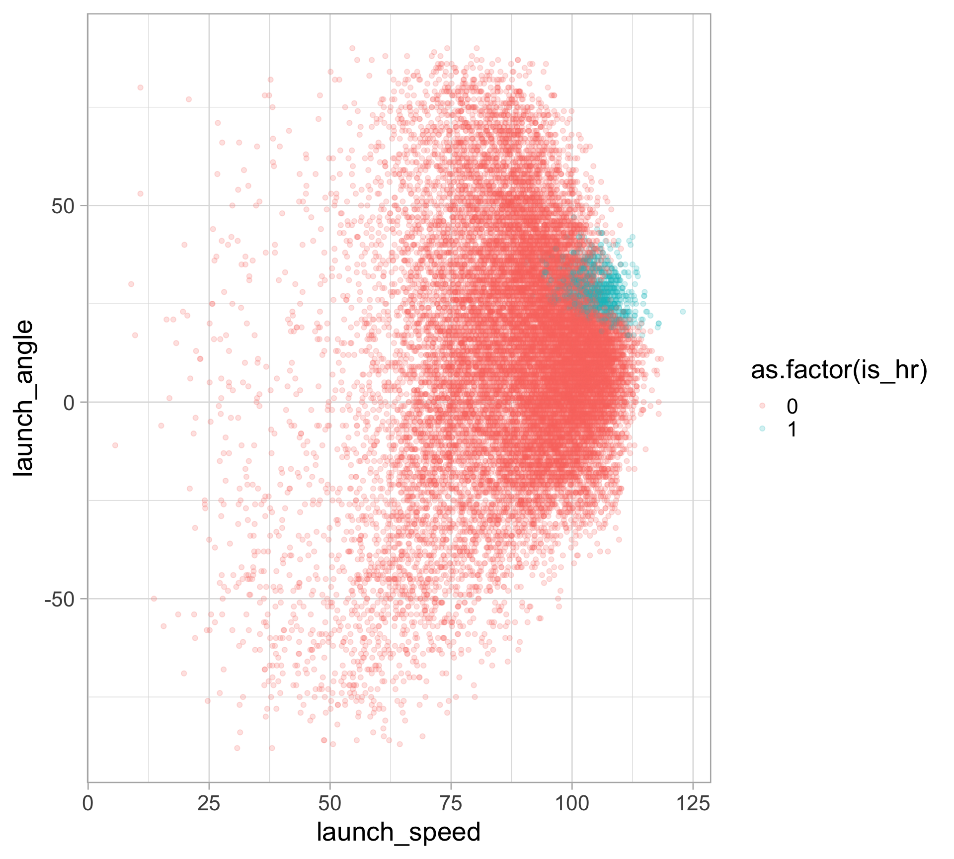

Predicting HRs with launch angle and exit velocity

There is a sweet spot of launch_angle (mid-way ish) and launch_speed (relatively high) where almost all HRs occur

batted_balls |> 
  group_by(
    launch_angle_bucket = round(launch_angle * 2, -1) / 2,
    launch_speed_bucket = round(launch_speed * 2, -1) / 2
  ) |> 
  summarize(hr = sum(is_hr == 1),
            n = n()) |> 
  ungroup() |> 
  mutate(pct_hr = hr / n) |> 
  ggplot(aes(x = launch_speed_bucket, 
             y = launch_angle_bucket, 
             fill = pct_hr)) +
  geom_tile() +
  scale_fill_gradient2(labels = scales::percent_format(),
                       low = "blue", 
                       high = "red", 
                       midpoint = 0.2)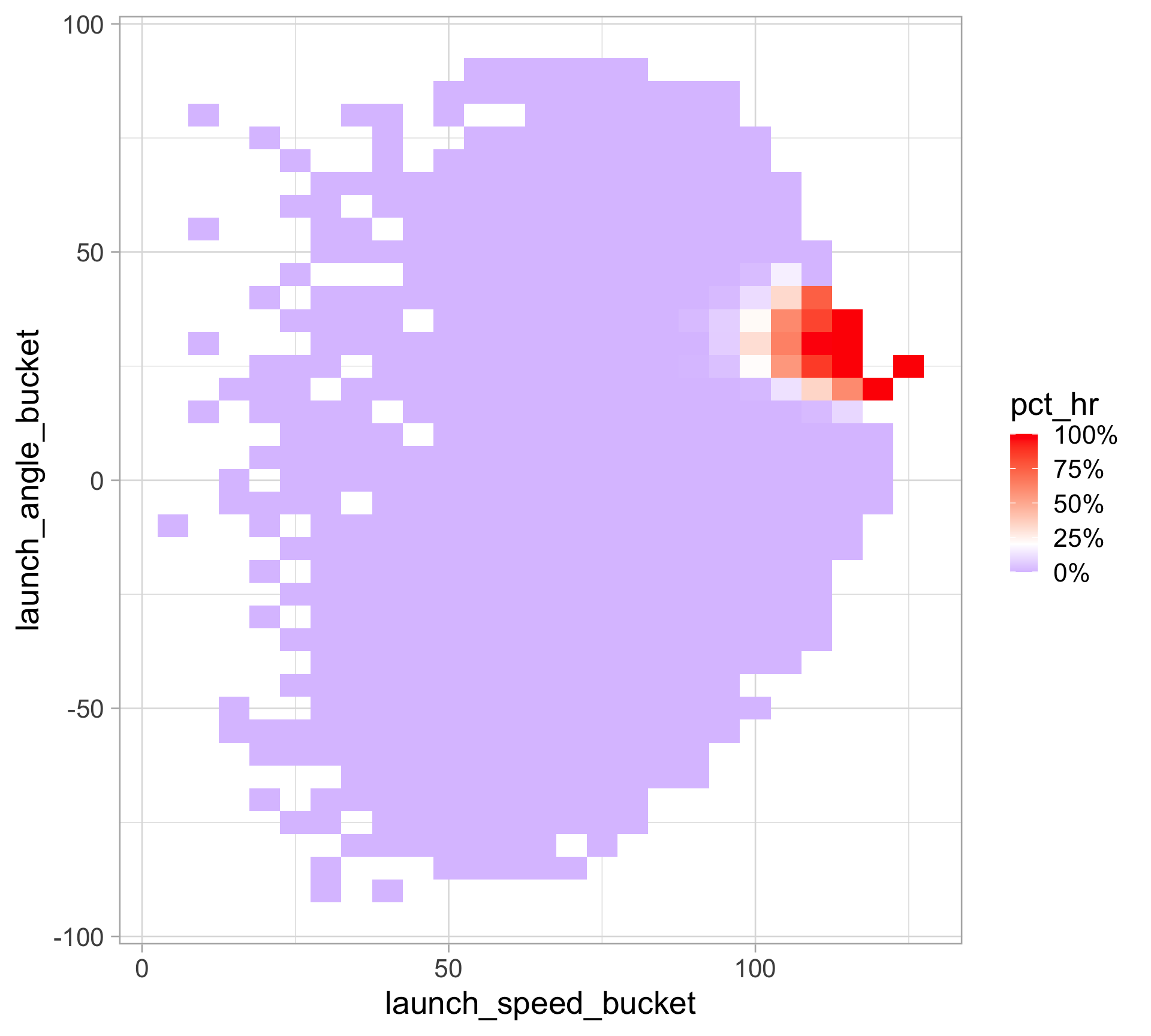

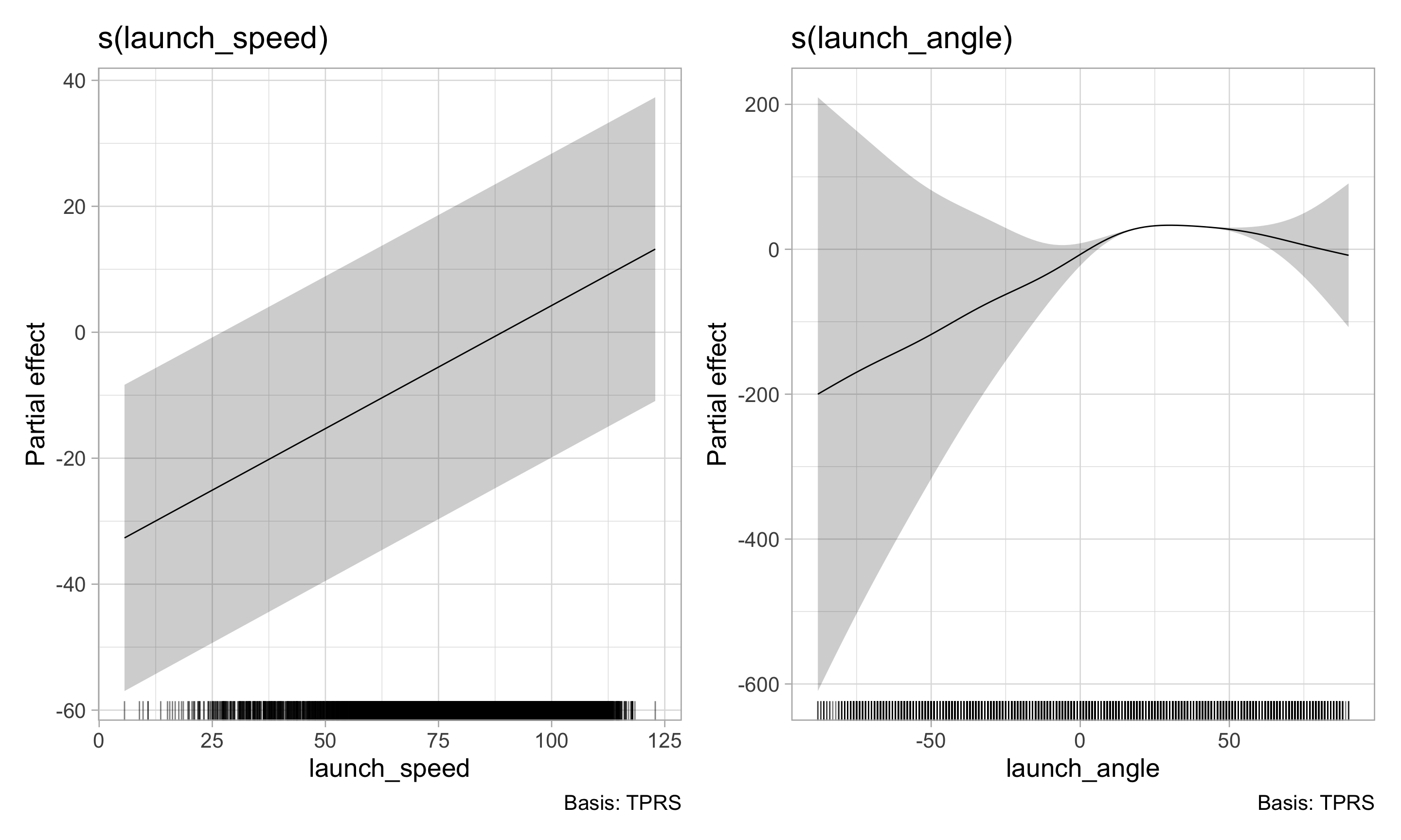
Fitting GAMs with mgcv

• Modeling the log-odds of a home run using non-linear functions of launch_speed and launch_angle \[ \log \left( \frac{p_{\texttt{is_hr}}}{1 - p_\texttt{is_hr}} \right) = \beta_0 + s_1 (\texttt{launch_speed}) + s_2 (\texttt{launch_angle})\] where \(p_\texttt{is_hr}\) is the probability of a home run

• Fit the model with smoothing spline functions s()

library(mgcv)
hr_gam <- gam(is_hr ~ s(launch_speed) + s(launch_angle),
              family = binomial,
              method = "REML", # more stable solution than default
              data = batted_balls)

View model summary

• mgcv performs hypothesis tests for the smooth terms — these are roughly the equivalent of an \(F\)-test for dropping each term

• Effective degrees of freedom (edf): basically the number of free parameters required to represent the function

• In a smoothing spline, different choices of \(\lambda\) correspond to different values of the edf, representing different amounts of smoothness

# summary(hr_gam)
library(broom)
# glance(hr_gam)
tidy(hr_gam)

# A tibble: 2 × 5
  term              edf ref.df statistic p.value
  <chr>           <dbl>  <dbl>     <dbl>   <dbl>
1 s(launch_speed)  1.00   1.00      804.       0
2 s(launch_angle)  3.73   3.98      468.       0

tidy(hr_gam, parametric = TRUE)

# A tibble: 1 × 5
  term        estimate std.error statistic p.value
  <chr>          <dbl>     <dbl>     <dbl>   <dbl>
1 (Intercept)    -38.3      12.3     -3.11 0.00189

Visualize partial response functions

Display the partial effect of each term in the model and how they add up to the overall prediction

library(gratia)
draw(hr_gam)

Model comparison: GAM vs GLM (logistic regression)

• 10-fold cross-validation: assigning games to folds

set.seed(25)
N_FOLDS <- 10
games_folds <- batted_balls |> 
  distinct(game_date, home_team, away_team) |>
  mutate(fold = sample(rep(1:N_FOLDS, length.out = n())))

batted_balls <- batted_balls |> 
  left_join(games_folds, by = join_by(game_date, home_team, away_team))

Cross-validation

hr_cv <- function(x) {
  hr_train <- batted_balls |> filter(fold != x)
  hr_test <- batted_balls |> filter(fold == x)
  
  gam_fit <- gam(is_hr ~ s(launch_speed) + s(launch_angle),
                 family = binomial,
                 method = "REML",
                 data = hr_train)
  logit_fit <- glm(is_hr ~ launch_speed + launch_angle, 
                   family = binomial, data = hr_train)
  
  hr_out <- tibble(
    gam_pred = predict(gam_fit, newdata = hr_test, type = "response"),
    logit_pred = predict(logit_fit, newdata = hr_test, type = "response"),
    test_actual = hr_test$is_hr,
    test_fold = x
  )
  return(hr_out)  
}

hr_preds <- map(1:N_FOLDS, hr_cv) |> 
  list_rbind()

Out-of-sample comparison

• Very few situations in reality where GLMs (with a linear predictor) perform better than an additive model using smooth functions

• Especially since smooth functions can just capture linear models

hr_preds |> 
  pivot_longer(cols = gam_pred:logit_pred, 
               names_to = "model", 
               values_to = "test_pred") |> 
  mutate(test_pred_class = round(test_pred)) |> 
  group_by(model, test_fold) |>
  summarize(accuracy = mean(test_pred_class == test_actual)) |> 
  group_by(model) |> 
  summarize(cv_accuracy = mean(accuracy),
            se_accuracy = sd(accuracy) / sqrt(N_FOLDS))

# A tibble: 2 × 3
  model      cv_accuracy se_accuracy
  <chr>            <dbl>       <dbl>
1 gam_pred         0.973     0.00105
2 logit_pred       0.959     0.00148

Appendix: code to build dataset

# pip install pybaseball
# dictionary: https://baseballsavant.mlb.com/csv-docs
import pandas as pd
from pybaseball import statcast
savant = statcast(start_dt='2025-05-01', end_dt='2025-05-31')
savant.to_csv('savant.csv', index=False)