Supervised learning: decision trees

SURE 2025

Department of Statistics & Data Science
Carnegie Mellon University

Background

Tree-based methods

• Can be applied to both regression and classification problems

• A single decision tree is simple and useful for interpretation

  • Main idea: partition/segment the predictor space into a number of simple regions

  • The set of splitting rules used to partition the predictor space can be summarized in a tree

• But decision trees generally do not have the same level of predictive performance as other methods

• Bagging, random forests, and boosting: grow multiple trees which are then combined to yield a single consensus prediction

• Combining a large number of trees can result in great improvements in prediction accuracy, at the expense of some loss interpretation

Regression trees: How do we partition?

Toy example: baseball salary

Regression trees

Fit a regression tree to predict the salary of a baseball player using

• Number of years they played in the major leagues

• Number of hits they made in the previous year

Regression trees

• At each node the label (e.g., \(X_j < t_k\) ) indicates that the left branch that comes from that split. The right branch is the opposite, e.g. \(X_j \geq t_k\).

• The first internal node indicates that those to the left have less than 4.5 years in the major league, on the right have \(\geq\) 4.5 years.

• The number on the top of the nodes indicates the predicted Salary, for example before doing any splitting, the average Salary for the whole dataset is 536 thousand dollars.

• This tree has two internal nodes and three termninal nodes

• This is probably an oversimplification, but it is very easy to interpret

Plotting a regression trees

Regression trees: partitioning the feature space

Regression trees: partitioning the feature space

Regression trees: partitioning the feature space

Terminology

• The final regions (1), (2) and (3) are called terminal nodes

• View the trees from upside down, the leaves are at the bottom

• The splits are called internal nodes

Decision tree: a more complex example

Decision tree structure

Decision tree structure

Predict the response value for an observation by following its path along the tree

(See previous baseball salary example)

• Decision trees are very easy to explain to non-statisticians.

• Easy to visualize and thus easy to interpret without assuming a parametric form

Tree-building process: the big picture

• Divide the predictor space (training data) into distinct and non-overlapping regions

  • The regions are found recursively using recursive binary splitting (i.e. asking a series of yes/no questions about the predictors)

  • Stop splitting the tree once a stopping criteria has been reached (e.g. maximum depth allowed)

• For a given region, make the same prediction for all observations in that region

  • Regression tree: the average of the response values in the node

  • Classification tree: the most popular class in the node

• Most popular algorithm: Classification and Regression Tree (CART)

Tree-building process: more details

• Divide the predictor space into high-dimensional rectangles (or boxes) - for simplicity and ease of interpretation

• Goal: find regions \(R_1, \dots, R_J\) that minimize the RSS

\[ \sum_{j=1}^J \sum_{i \in R_j} (y_i - \hat y_{R_j})^2 \]

where \(\hat y_{R_j}\) is the mean response for the training observations within the \(j\)th region (at the terminal node)

• So observations within each region are similar (basically having the same predicted response), and observations across regions are different

• Challenge: it is computationally infeasible to consider every possible partition of the feature space into \(J\) regions

Tree-building process: more details

Solution: recursive binary splitting (a top-down, greedy approach)

• top-down

  • begin at the top of the tree

  • then successively split the predictor space

  • each split is indicated via two new branches further down on the tree

• greedy

  • at each step of the tree-building process, the best split is made at that particular step

  • rather than looking ahead and picking a split that will lead to a better tree in some future step

Tree-building process: more details

• First, select predictor \(X_j\) and cutpoint \(s\) such that

  • splitting the predictor space into the regions \(\{X \mid X_j < s\}\) and \(\{X \mid X_j \ge s\}\) will yield the greatest possible reduction in RSS

• Next, repeat the process

  • looking for the best predictor and best cutpoint in order to split the data further

  • so as to minimize the RSS within each of the resulting regions

  • BUT…split one of the two previously identified region (instead of the entire predictor space)

• Continue the process until a stopping criterion is reached (i.e. how complex should the tree be?)

  • maximum tree depth

  • minimum node size

Pruning a tree

• The process described above may produce good training performance but poor test set performance (i.e. overfitting)

• A smaller tree with fewer splits (i.e. fewer regions \(R_1, \dots, R_J\)): low variance, high bias

• A larger tree with more splits: high variance, low bias

• Solution: tree pruning

  • Grow a very large complicated tree

  • Then prune back to an optimal subtree

• Tuning parameter: cost complexity parameter \(\alpha\)

  • Minimize \[\text{RSS} + \alpha \vert T \vert\] where \(\vert T \vert\) is the number of terminal nodes of the tree \(T\)

  • Controls a trade-off between the subtree’s complexity and its fit to the training data

  • How do we select the optimal value?

Summary: regression tree algorithm

1. Use recursive binary splitting to grow a large tree on the training data, stopping only when each terminal node has fewer than some minimum number of observations

2. Apply cost complexity pruning to the large tree in order to obtain a sequence of best subtrees, as a function of \(\alpha\)

3. Use \(K\)-fold cross-validation to choose \(\alpha\)

4. Return the subtree from Step 2 that corresponds to the optimal chosen value of \(\alpha\)

Classification trees

• What if the response is categorical?

• Predict that each observation belongs to the most commonly occurring class in the region to which it belongs

• Just like regression trees, use recursive binary splitting to grow a classification tree

• But we need a different criterion for making the binary splits other than RSS

Classification trees

• Instead of RSS, use the Gini index \[G = \sum_{k=1}^K \hat p_{jk} (1 - \hat p_{jk})\] where \(\hat p_{jk}\) is proportion of observations in the \(j\)th region that are from the \(k\)th class

• A measure of total variance across the \(K\) classes

• A measure of node purity (or node impurity)

  • small value: a node contains mostly observations from a single class

• Alternative measure: cross-entropy

\[G = - \sum_{k=1}^K \hat p_{jk} \log\hat p_{jk} \]

Examples

Predicting MLB home run probability

library(tidyverse)
theme_set(theme_light())
batted_balls <- read_csv("https://raw.githubusercontent.com/36-SURE/2025/main/data/batted_balls.csv") |> 
  mutate(is_hr = as.factor(is_hr))
glimpse(batted_balls)

Rows: 20,188
Columns: 14
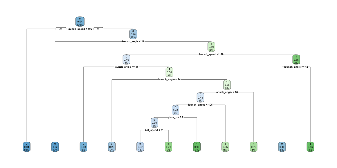
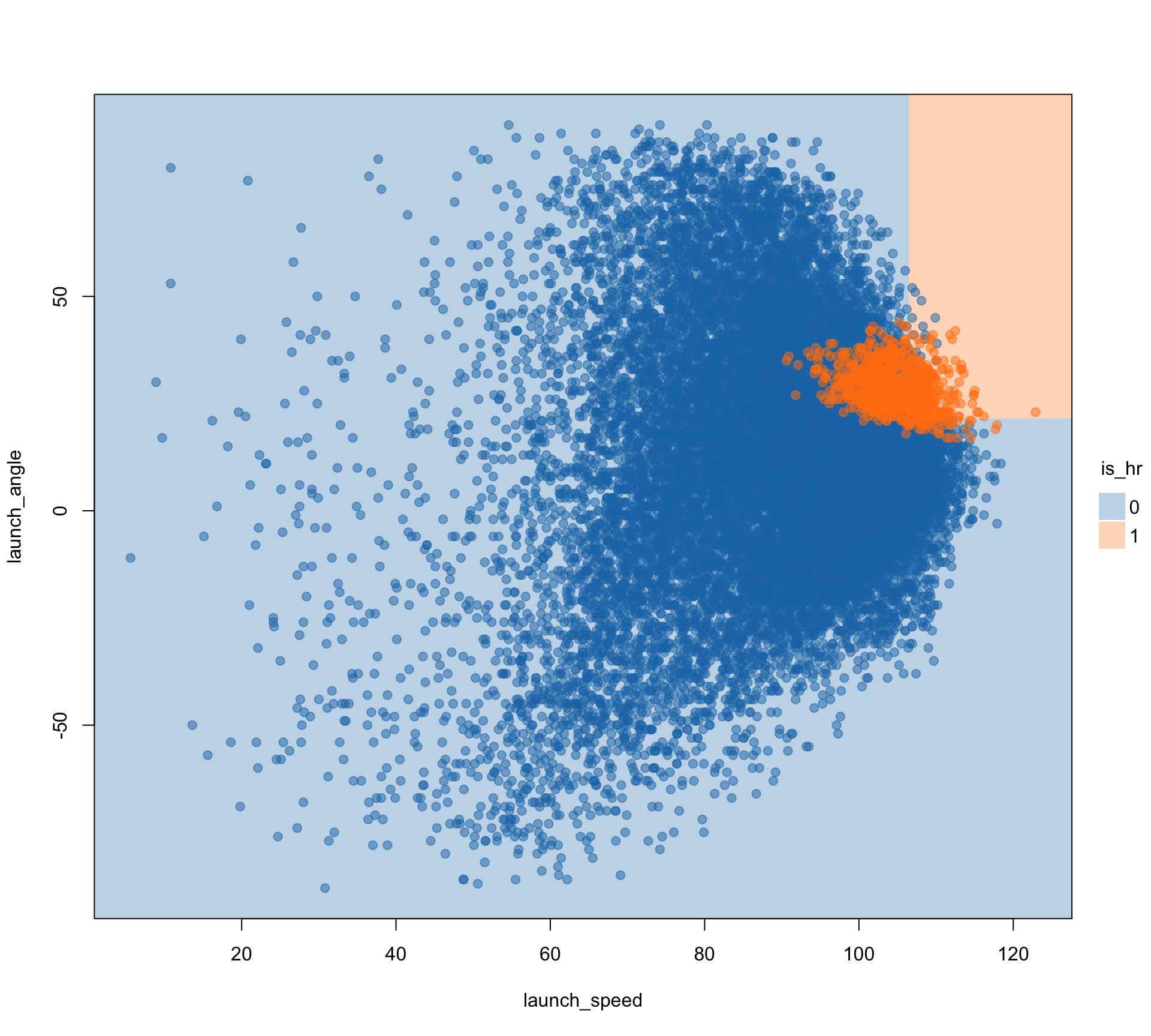
$ is_hr           <fct> 0, 0, 0, 0, 0, 0, 0, 0, 0, 0, 0, 0, 0, 0, 0, 0, 0, 0, …
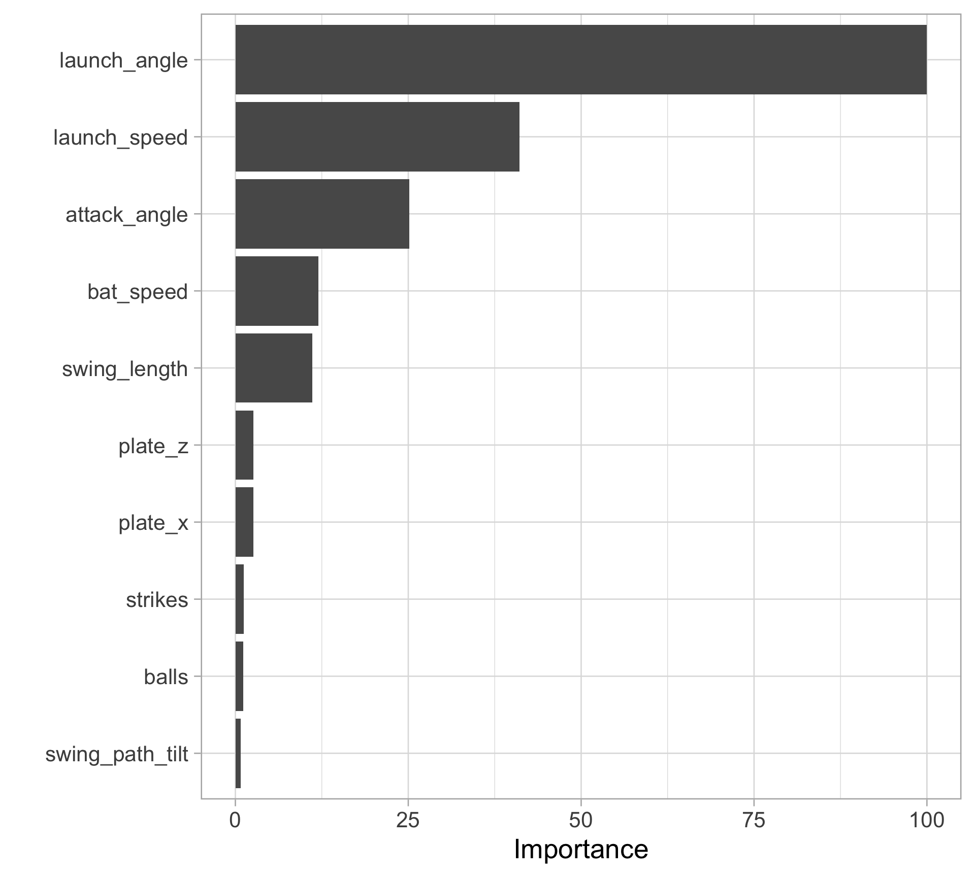
$ launch_angle    <dbl> 33, -20, 36, 4, 20, 28, 27, 12, 8, -25, 16, 50, 68, 7,…
$ launch_speed    <dbl> 91.3, 71.4, 103.4, 100.8, 102.3, 90.4, 90.4, 76.9, 101…
$ bat_speed       <dbl> 76.3, 79.2, 72.3, 72.2, 67.8, 79.1, 74.7, 70.4, 74.3, …
$ swing_length    <dbl> 8.2, 8.0, 6.4, 8.4, 5.9, 7.7, 8.2, 6.6, 7.0, 6.7, 6.6,…
$ attack_angle    <dbl> 0.1394548, 22.2024920, 11.7628706, 3.3512694, -4.21284…
$ swing_path_tilt <dbl> 40.20981, 30.55564, 29.29605, 29.01934, 26.56705, 33.4…
$ plate_x         <dbl> -0.45, 0.26, -0.04, -0.65, -0.40, -0.25, -0.23, -0.94,…
$ plate_z         <dbl> 1.98, 2.02, 2.75, 1.81, 2.78, 2.08, 1.58, 2.14, 2.70, …
$ inning          <dbl> 9, 9, 9, 8, 8, 8, 8, 7, 7, 6, 6, 6, 5, 5, 5, 5, 5, 5, …
$ balls           <dbl> 0, 1, 3, 2, 0, 1, 1, 2, 3, 0, 0, 2, 0, 2, 0, 1, 0, 0, …
$ strikes         <dbl> 2, 2, 2, 1, 0, 2, 2, 2, 2, 0, 0, 2, 0, 2, 0, 1, 1, 1, …
$ is_stand_left   <dbl> 1, 0, 1, 1, 1, 1, 0, 0, 1, 1, 1, 1, 0, 1, 0, 1, 0, 1, …
$ is_throw_left   <dbl> 0, 0, 0, 0, 0, 1, 1, 0, 0, 1, 0, 0, 0, 0, 0, 0, 0, 0, …

Model training with caret

library(caret)
set.seed(10)
hr_tree <- train(is_hr ~ ., method = "rpart", tuneLength = 20,
                 trControl = trainControl(method = "cv", number = 10),
                 data = batted_balls)
# str(hr_tree)
ggplot(hr_tree)

Display the final tree model with rpart.plot

library(rpart.plot)
hr_tree |> 
  pluck("finalModel") |> 
  rpart.plot()

Variable importance

• Recall that in a binary decision tree, at each node, a single predictor is used to partition the data into two homogeneous groups.

• The chosen predictor is the one that maximizes some measure of improvement (e.g. RSS, Gini index)

• The relative importance of predictor \(X^*\) is the sum of the squared improvements over all internal nodes of the tree for which \(X\) was chosen as the partitioning variable

Variable importance with vip

library(vip)
hr_tree |> 
  vip()

More visualization with parttree

• For illustration purpose only, since this only works for models with one or two predictors

library(parttree)
hr_simple_tree <- rpart(
  is_hr ~ launch_speed + launch_angle,
  data = batted_balls
)

hr_simple_tree |> 
  parttree() |> 
  plot(palette = "classic", 
       alpha = 0.5, 
       pch = 19,
       border = NA)

Bonus: treemaps for visualizing categorical data

• Note: this has nothing to do with the lecture content

• But is a cool way to visualize categorical data, as an alternative to mosaic plots

• Treemaps do not require the same categorical levels across subgroups

library(treemapify)
penguins |>
  count(species, island) |>
  ggplot(aes(area = n, subgroup = island, label = species,
             fill = interaction(species, island))) +
  # draw species borders and fill colors
  geom_treemap() +
  # draw island borders
  geom_treemap_subgroup_border() +
  # print island text
  geom_treemap_subgroup_text(
    place = "center", grow = TRUE, alpha = 0.5, 
    color = "black", fontface = "italic", min.size = 0
  )+
  # print species text
  geom_treemap_text(color = "white", place = "topleft", 
                    reflow = TRUE) +
  guides(color = "none", fill = "none")

Bonus: waffle charts

• Again, not related to the lecture content, but another cool way to visualize categorical data

library(waffle)
penguins |>
  count(species) |>
  ggplot(mapping = aes(fill = species, values = n)) +
  geom_waffle(size = 1, color = "white",
              make_proportional = TRUE) +
  scale_fill_viridis_d(end = 0.8) +
  labs(title = "Penguins by species",
       x = NULL, y = NULL, fill = NULL) +
  coord_equal() +
  theme_void() +
  theme(legend.position = "top")

Appendix: code to build dataset

savant <- read_csv("https://raw.githubusercontent.com/36-SURE/2025/main/data/savant.csv")
batted_balls <- savant |> 
  filter(type == "X") |> 
  mutate(is_hr = as.numeric(events == "home_run"),
         is_stand_left = as.numeric(stand == "L"),
         is_throw_left = as.numeric(p_throws == "L")) |> 
  filter(!is.na(launch_angle), !is.na(launch_speed), !is.na(is_hr)) |> 
  select(is_hr, launch_angle, launch_speed, bat_speed, swing_length, 
         attack_angle, swing_path_tilt, plate_x, plate_z, 
         inning, balls, strikes, is_stand_left, is_throw_left) |> 
  drop_na()