Exploring data: into the `tidyverse`

CMSACamp 2026

Department of Statistics & Data Science
Carnegie Mellon University

Data science workflow

Workflow diagram

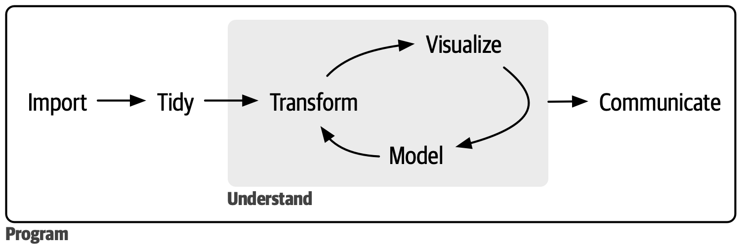
First few lectures: data wrangling and data visualization
Aspects of data wrangling:
- Import: load in data (e.g., read_csv())
- Tidy: each row is an observation, each column is a variable (i.e. tabular data)
- Transform: filter observations, create new variables, etc.

Exploratory data analysis

Goal of EDA: perform initial investigations on the data to better understand the data, discover trends/patterns, spot anomalies, etc.

“EDA is an iterative cycle”
- Generate questions about data
- Answer via data wrangling and visualization

“EDA is a state of mind”

Exploratory data analysis

Data can be explored numerically (tables, descriptive statistics, etc.) or visually (graphs)
Examples of questions:
- What type of variation do the variables display?
- What type of relationships exist between variables?

EDA is NOT a replacement for statistical inference and learning

EDA is an important and necessary step to build intuition

First example: MLB batting statistics

Import Batting table of historical MLB batting statistics from the Lahman package.

library(tidyverse) # load the tidyverse
library(Lahman) # load the Lahman package to access its datasets
Batting <- as_tibble(Batting) # initialize the Batting dataset

Basic info about the Batting dataset:

# number of rows and columns
# can also do nrow(Batting) and ncol(Batting)
dim(Batting)

[1] 128598     22

class(Batting)

[1] "tbl_df"     "tbl"        "data.frame"

First example: MLB batting statistics

Always look at your data: view the first 6 (by default) rows with head()

# try just typing Batting into your console, what happens? Also try glimpse(Batting)
head(Batting)

# A tibble: 6 × 22
  playerID  yearID stint teamID lgID      G    AB     R     H   X2B   X3B    HR
  <chr>      <int> <int> <fct>  <fct> <int> <int> <int> <int> <int> <int> <int>
1 aardsda01   2004     1 SFN    NL       11     0     0     0     0     0     0
2 aardsda01   2006     1 CHN    NL       45     2     0     0     0     0     0
3 aardsda01   2007     1 CHA    AL       25     0     0     0     0     0     0
4 aardsda01   2008     1 BOS    AL       47     1     0     0     0     0     0
5 aardsda01   2009     1 SEA    AL       73     0     0     0     0     0     0
6 aardsda01   2010     1 SEA    AL       53     0     0     0     0     0     0
# ℹ 10 more variables: RBI <int>, SB <int>, CS <int>, BB <int>, SO <int>,
#   IBB <int>, HBP <int>, SH <int>, SF <int>, GIDP <int>

Is the Batting dataset tidy?

Each row = a player’s season stint with a team (i.e. players can play for multiple teams in year)
Each column = different measurement or recording about the player-team-season observation (get all column names with colnames(Batting) or names(Batting))

Descriptive statistics

We summarize quantitative (e.g. yearID, AB) and categorical (e.g. teamID, lgID) variables in different ways

Compute summary statistics for quantitative variables with the summary() function:

summary(Batting$G)

   Min. 1st Qu.  Median    Mean 3rd Qu.    Max. 
    1.0    11.0    31.0    47.3    71.0   165.0

Compute counts of categorical variables with the table() function:

# be careful it ignores NA values!
# can do table(Batting$lgID, useNA = "always")
table(Batting$lgID)


   AA    AL   ANL   EAS   ECL   EWL    FL   IND   INT    NA   NAC   NAL    NL 
 1893 54277   154  1035   917   191   472   827    44   737   105  2114 59279 
  NN2   NNL   NSL    PL    UA   WES 
 2731  2275   237   149   334   827

Data wrangling with `dplyr`

The `dplyr` package

dplyr is a package within the tidyverse with functions for data wrangling

“Grammar of data manipulation”:

dplyr functions are verbs
datasets are nouns
function arguments are adverbs

The six main dplyr verbs for data wrangling:

filter()
select()
arrange()
mutate()
group_by()
summarize()

`filter()`

We can use filter() to extract rows (i.e. observations) that meet certain conditions

Note: These conditions must be logical conditions (aka boolean expressions)

`filter()`

Example 1: Extract batting stats for the American League (AL) and National League (NL)

mlb_batting <- filter(Batting, lgID %in% c("AL", "NL")) # or filter(Batting, lgID == "AL" | lgID == "NL")
nrow(Batting) - nrow(mlb_batting) # difference in row counts

[1] 15042

Example 2: Extract batting stats for Pirates players in 2022

# multiple conditions
pirates_batting <- filter(Batting, yearID == 2022 & teamID == "PIT")
head(pirates_batting, n = 3) # difference in row counts

# A tibble: 3 × 22
  playerID  yearID stint teamID lgID      G    AB     R     H   X2B   X3B    HR
  <chr>      <int> <int> <fct>  <fct> <int> <int> <int> <int> <int> <int> <int>
1 alforan01   2022     1 PIT    NL        2     4     0     1     0     0     0
2 alldrca01   2022     1 PIT    NL        1     0     0     0     0     0     0
3 allengr01   2022     1 PIT    NL       46   118    17    22     4     0     2
# ℹ 10 more variables: RBI <int>, SB <int>, CS <int>, BB <int>, SO <int>,
#   IBB <int>, HBP <int>, SH <int>, SF <int>, GIDP <int>

Logical conditions

x < y: less than
x <= y: less than or equal to
x == y: equal to
x != y: not equal to
x > y: greater than
x >= y: greater than or equal to

x %in% y: whether the value is present in a given vector
is.na(x): is missing
x & y: and
x | y: or
!x: not

… and basically anything that returns a TRUE/FALSE value

Common mistakes

Using = instead of ==

nay

filter(Batting, team = "PIT")

yay

filter(Batting, team == "PIT")

Forgetting quotes (for string/character)

nay

filter(Batting, team == PIT)

yay

filter(Batting, team == "PIT")

`select()`

We can use select() to extract columns (variables) of interest

We simply specify the column names:

select(Batting, playerID, yearID, G, AB, R, H, HR, BB)

# A tibble: 128,598 × 8
   playerID  yearID     G    AB     R     H    HR    BB
   <chr>      <int> <int> <int> <int> <int> <int> <int>
 1 aardsda01   2004    11     0     0     0     0     0
 2 aardsda01   2006    45     2     0     0     0     0
 3 aardsda01   2007    25     0     0     0     0     0
 4 aardsda01   2008    47     1     0     0     0     0
 5 aardsda01   2009    73     0     0     0     0     0
 6 aardsda01   2010    53     0     0     0     0     0
 7 aardsda01   2012     1     0     0     0     0     0
 8 aardsda01   2013    43     0     0     0     0     0
 9 aardsda01   2015    33     1     0     0     0     0
10 aaronha01   1954   122   468    58   131    13    28
# ℹ 128,588 more rows

`mutate()`

We use mutate() to create new variables

New variables created via mutate() are usually based on existing variables
Make sure to give your new variable a name
Naming the new variable the same as the existing variable will overwrite the original column

Example: Get the batting average and strikeout-to-walk ratio for every player

new_batting <- mutate(Batting, batting_avg = H / AB, so_bb_ratio = SO / BB)
head(new_batting, n = 1)

# A tibble: 1 × 24
  playerID  yearID stint teamID lgID      G    AB     R     H   X2B   X3B    HR
  <chr>      <int> <int> <fct>  <fct> <int> <int> <int> <int> <int> <int> <int>
1 aardsda01   2004     1 SFN    NL       11     0     0     0     0     0     0
# ℹ 12 more variables: RBI <int>, SB <int>, CS <int>, BB <int>, SO <int>,
#   IBB <int>, HBP <int>, SH <int>, SF <int>, GIDP <int>, batting_avg <dbl>,
#   so_bb_ratio <dbl>

`arrange()`

We use arrange() to sort the observations (rows) by variables (columns)

Default is ascending order:

Low to high for numeric columns
Alphabetical order for character columns

Example 1: Who holds the single-season home run record?

hr_batting <- arrange(Batting, desc(HR)) # desc() for descending order
head(hr_batting, n = 3)

# A tibble: 3 × 22
  playerID  yearID stint teamID lgID      G    AB     R     H   X2B   X3B    HR
  <chr>      <int> <int> <fct>  <fct> <int> <int> <int> <int> <int> <int> <int>
1 bondsba01   2001     1 SFN    NL      153   476   129   156    32     2    73
2 mcgwima01   1998     1 SLN    NL      155   509   130   152    21     0    70
3 sosasa01    1998     1 CHN    NL      159   643   134   198    20     0    66
# ℹ 10 more variables: RBI <int>, SB <int>, CS <int>, BB <int>, SO <int>,
#   IBB <int>, HBP <int>, SH <int>, SF <int>, GIDP <int>

`arrange()`

Example 2: we can arrange by multiple columns at once:

At bats from high to low
Home runs from low to high

Variable order matters!

ab_hr_batting <- arrange(Batting, desc(AB), HR)
head(ab_hr_batting, n = 3)

# A tibble: 3 × 22
  playerID  yearID stint teamID lgID      G    AB     R     H   X2B   X3B    HR
  <chr>      <int> <int> <fct>  <fct> <int> <int> <int> <int> <int> <int> <int>
1 rolliji01   2007     1 PHI    NL      162   716   139   212    38    20    30
2 wilsowi02   1980     1 KCA    AL      161   705   133   230    28    15     3
3 suzukic01   2004     1 SEA    AL      161   704   101   262    24     5     8
# ℹ 10 more variables: RBI <int>, SB <int>, CS <int>, BB <int>, SO <int>,
#   IBB <int>, HBP <int>, SH <int>, SF <int>, GIDP <int>

Performing multiple operations

What if we want to perform several tasks using multiple dplyr verbs?

Example: Which Pirates players had the highest batting average in 2022, among those with at least 50 at bats?

select(arrange(mutate(filter(Batting, yearID == 2022, teamID == "PIT", AB >= 50), batting_avg = H / AB), desc(batting_avg)), playerID, AB, batting_avg)

# A tibble: 23 × 3
   playerID     AB batting_avg
   <chr>     <int>       <dbl>
 1 newmake01   288       0.274
 2 reynobr01   542       0.262
 3 hayeske01   505       0.244
 4 marisja01    77       0.234
 5 perezro02    60       0.233
 6 castrro01   253       0.233
 7 cruzon01    331       0.233
 8 gamelbe01   371       0.232
 9 chavimi01   401       0.229
10 vogelda01   237       0.228
# ℹ 13 more rows

That’s awfully annoying to write, and also difficult to read…

The pipe operator

Introducing the pipe operator |>

Note: You might have seen the magrittr pipe %>%…

This is from the maggritr package, automatically loaded when loading tidyverse
Recently, many people (including Hadley Wickham) have switched to |>, the built-in “native” pipe to base R
While identical in many ways, there are some differences

The pipe operator

We use |> to perform a sequence of operations (think of as: “and then…”)
The pipe takes an object (e.g., tibble, data frame, matrix, vector) on the left and passes it as the first argument of the function on the right

# the workflow
object |>
  first_operation(...) |>
  second_operation(...) |> 
  .
  .
  .
  last_operation(...)

Performing multiple operations

Recall our example: Which Pirates players had the highest batting average in 2022, among those with at least 50 at bats?

Our list of tasks:

filter(): only Pirates players in 2022 with at least 50 at bats
mutate(): create a new column for batting average
arrange(): sort by batting average in descending order
select(): report player name, at bats, and batting average

Performing multiple operations

Batting |> 
  filter(yearID == 2022, teamID == "PIT", AB >= 50) |> 
  mutate(batting_avg = H / AB) |> 
  arrange(desc(batting_avg)) |> 
  select(playerID, AB, batting_avg)

# A tibble: 23 × 3
   playerID     AB batting_avg
   <chr>     <int>       <dbl>
 1 newmake01   288       0.274
 2 reynobr01   542       0.262
 3 hayeske01   505       0.244
 4 marisja01    77       0.234
 5 perezro02    60       0.233
 6 castrro01   253       0.233
 7 cruzon01    331       0.233
 8 gamelbe01   371       0.232
 9 chavimi01   401       0.229
10 vogelda01   237       0.228
# ℹ 13 more rows

This is much easier to write and read!

`summarize()` (by itself)

We use summarize() to collapse the data down to a single row (per group) by aggregating variables into single values

This is useful for computing summaries (e.g., mean, median, max, min, correlation)

Example 1: Extracting the median at bats

Batting |> 
  summarize(median_at_bats = median(AB))

# A tibble: 1 × 1
  median_at_bats
           <dbl>
1             40

Example 2: Extracting the correlation between at bats and home runs

Batting |> 
  summarize(cor_ab_hr = cor(AB, HR))

# A tibble: 1 × 1
  cor_ab_hr
      <dbl>
1     0.712

`group_by()` and `summarize()`

We can use group_by() to covert the data into a “grouped tbl”, where operations are performed by group

That is, group_by() splits the data into groups based on column values
Powerful when combined with summarize()
After the operation is done at the group-level, you may have to use ungroup() to remove leftover groupings

`group_by()` and `summarize()`

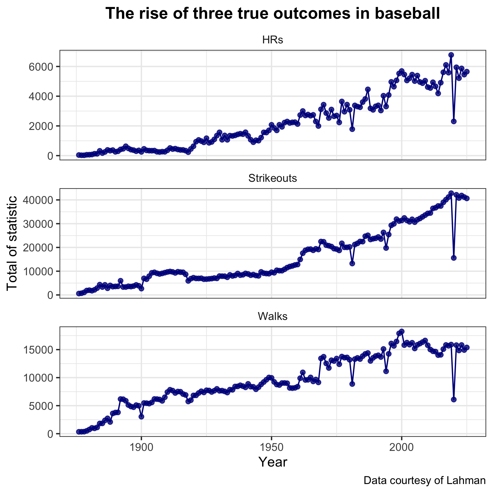
Example: How many home runs, strike outs, and walks did each team accumulate in each season from 2015 to 2019?

Batting |> 
  filter(yearID %in% 2015:2019) |> 
  group_by(teamID) |> 
  summarize(total_hr = sum(HR), total_so = sum(SO), total_bb = sum(BB)) |> 
  arrange(desc(total_hr))

# A tibble: 30 × 4
   teamID total_hr total_so total_bb
   <fct>     <int>    <int>    <int>
 1 NYA        1209     6659     2839
 2 HOU        1159     6294     2759
 3 TOR        1139     6741     2752
 4 LAN        1111     6751     2991
 5 BAL        1103     6914     2162
 6 TEX        1041     7008     2572
 7 SEA        1036     6693     2489
 8 MIN        1035     6694     2604
 9 OAK        1033     6474     2610
10 MIL        1031     7434     2724
# ℹ 20 more rows

The lesser-known stars of `dplyr`

`count()`

count() returns the number of observations in each group

Batting |> 
  count(lgID, name = "freq")

# A tibble: 19 × 2
   lgID   freq
   <fct> <int>
 1 AA     1893
 2 AL    54277
 3 ANL     154
 4 EAS    1035
 5 ECL     917
 6 EWL     191
 7 FL      472
 8 IND     827
 9 INT      44
10 NA      737
11 NAC     105
12 NAL    2114
13 NL    59279
14 NN2    2731
15 NNL    2275
16 NSL     237
17 PL      149
18 UA      334
19 WES     827

Alternatives to `count()`

Using group_by() and summarize()

# note: count is a "shortcut" of this
Batting |> 
  group_by(lgID) |> 
  summarize(freq = n()) |> 
  ungroup()

Using Base R

# recall that in base R...
table(Batting$lgID)

`slice_*()` family for subsetting rows

slice(): extract rows (observations) based on the row index

Batting |> 
  slice(c(1, 99, 101, 500))

# A tibble: 4 × 22
  playerID  yearID stint teamID lgID      G    AB     R     H   X2B   X3B    HR
  <chr>      <int> <int> <fct>  <fct> <int> <int> <int> <int> <int> <int> <int>
1 aardsda01   2004     1 SFN    NL       11     0     0     0     0     0     0
2 abbotfr01   1904     1 CLE    AL       41   130    14    22     4     2     0
3 abbotgl01   1973     1 OAK    AL        5     0     0     0     0     0     0
4 adamsbo03   1951     1 CIN    NL      125   403    57   107    12     5     5
# ℹ 10 more variables: RBI <int>, SB <int>, CS <int>, BB <int>, SO <int>,
#   IBB <int>, HBP <int>, SH <int>, SF <int>, GIDP <int>

`slice_*()` family for subsetting rows

slice_head() / slice_tail(): extract the first / last n rows

# Batting |> slice_tail(n = 5)
Batting |> 
  slice_head(n = 5)

# A tibble: 5 × 22
  playerID  yearID stint teamID lgID      G    AB     R     H   X2B   X3B    HR
  <chr>      <int> <int> <fct>  <fct> <int> <int> <int> <int> <int> <int> <int>
1 aardsda01   2004     1 SFN    NL       11     0     0     0     0     0     0
2 aardsda01   2006     1 CHN    NL       45     2     0     0     0     0     0
3 aardsda01   2007     1 CHA    AL       25     0     0     0     0     0     0
4 aardsda01   2008     1 BOS    AL       47     1     0     0     0     0     0
5 aardsda01   2009     1 SEA    AL       73     0     0     0     0     0     0
# ℹ 10 more variables: RBI <int>, SB <int>, CS <int>, BB <int>, SO <int>,
#   IBB <int>, HBP <int>, SH <int>, SF <int>, GIDP <int>

`slice_*()` family for subsetting rows

slice_min() / slice_max(): extract rows with the smallest or largest values of a variable

# single-season home run record (top 5)
Batting |> 
  slice_max(HR, n = 5)

# A tibble: 5 × 22
  playerID  yearID stint teamID lgID      G    AB     R     H   X2B   X3B    HR
  <chr>      <int> <int> <fct>  <fct> <int> <int> <int> <int> <int> <int> <int>
1 bondsba01   2001     1 SFN    NL      153   476   129   156    32     2    73
2 mcgwima01   1998     1 SLN    NL      155   509   130   152    21     0    70
3 sosasa01    1998     1 CHN    NL      159   643   134   198    20     0    66
4 mcgwima01   1999     1 SLN    NL      153   521   118   145    21     1    65
5 sosasa01    2001     1 CHN    NL      160   577   146   189    34     5    64
# ℹ 10 more variables: RBI <int>, SB <int>, CS <int>, BB <int>, SO <int>,
#   IBB <int>, HBP <int>, SH <int>, SF <int>, GIDP <int>

`slice_*()` family for subsetting rows

slice_sample(): randomly sample a specified number / fraction of observation in the data

# randomly sample 1000 rows (without replacement, by default)
Batting |> 
  slice_sample(n = 1000)

# randomly sample 70% of the rows, with replacement
Batting |> 
  slice_sample(prop = 0.7, replace = TRUE)

Useful for performing resampling (e.g., bootstrap, cross-validation, etc.)

Putting it all together (pt. 2)

Example 1: Get batting stats for each year: each row is a year with the following variables

total hits, home runs, strikeouts, walks, atbats
total batting average for each year = total H / total AB
only keeps AL and NL leagues

yearly_batting <- Batting |>
  filter(lgID %in% c("AL", "NL")) |>
  group_by(yearID) |>
  summarize(total_h = sum(H, na.rm = TRUE),
            total_hr = sum(HR, na.rm = TRUE),
            total_so = sum(SO, na.rm = TRUE),
            total_bb = sum(BB, na.rm = TRUE),
            total_ab = sum(AB, na.rm = TRUE)) |>
  mutate(batting_avg = total_h / total_ab)

Putting it all together (pt. 2)

Example 2: What are the top three years with the most HRs?

yearly_batting |> 
  slice_max(total_hr, n = 3)

# A tibble: 3 × 7
  yearID total_h total_hr total_so total_bb total_ab batting_avg
   <int>   <int>    <int>    <int>    <int>    <int>       <dbl>
1   2019   42039     6776    42823    15895   166651       0.252
2   2017   42215     6105    40104    15829   165567       0.255
3   2021   39484     5944    42145    15794   161941       0.244

# or this 
yearly_batting |>
  arrange(desc(total_hr)) |>
  slice(1:3)

# A tibble: 3 × 7
  yearID total_h total_hr total_so total_bb total_ab batting_avg
   <int>   <int>    <int>    <int>    <int>    <int>       <dbl>
1   2019   42039     6776    42823    15895   166651       0.252
2   2017   42215     6105    40104    15829   165567       0.255
3   2021   39484     5944    42145    15794   161941       0.244

Putting it all together (pt. 2)

Example 3: Which years have the best and worst strikeout to walk ratios?

yearly_batting |>
  mutate(so_bb_ratio = total_so / total_bb) |>
  arrange(so_bb_ratio) |>
  slice(c(1, n()))

# A tibble: 2 × 8
  yearID total_h total_hr total_so total_bb total_ab batting_avg so_bb_ratio
   <int>   <int>    <int>    <int>    <int>    <int>       <dbl>       <dbl>
1   1893   15913      460     3341     6143    56898       0.280       0.544
2   1879    6171       58     1843      508    24155       0.255       3.63

We can make better looking tables

Using rename() and gt():

library(gt)

yearly_batting |>
  select(yearID, batting_avg) |>
  rename(Year = yearID, `Batting Average` = batting_avg) |>
  arrange(desc(`Batting Average`)) |>
  slice(c(1:3, (n()-2):n())) |>
  gt() |>
  fmt_number(columns = `Batting Average`, decimals = 3)

Year	Batting Average
1894	0.309
1895	0.296
1930	0.296
1908	0.239
1888	0.239
1968	0.237

Lots of ways to customize tables with `gt()`

yearly_batting |>
  select(yearID, batting_avg) |>
  rename(Year = yearID,
         `Batting Average` = batting_avg) |>
  arrange(desc(`Batting Average`)) |>
  slice(c(1:3, (n()-2):n())) |>
  gt(rowname_col = "Year") |>
  # add table header
  tab_header(title = "Best / Worst MLB Seasons by Batting Average") |>
  # create row groups by location 
  tab_row_group(
    label = "Bottom 3 Years",
    rows = 4:6
  ) |>
  tab_row_group(
    label = "Top 3 Years",
    rows = 1:3
  ) |>
  # recolor row group labels
  tab_style(
    style = cell_fill(color = "bisque"),
    locations = cells_row_groups(groups = "Bottom 3 Years")
  ) |>
  tab_style(
    style = cell_fill(color = "darkseagreen1"),
    locations = cells_row_groups(groups = "Top 3 Years")) |>
  # round "Batting Average" to 3 decimals 
  fmt_number(columns = `Batting Average`, decimals = 3)

	Batting Average
Best / Worst MLB Seasons by Batting Average
Top 3 Years
1894	0.309
1895	0.296
1930	0.296
Bottom 3 Years
1908	0.239
1888	0.239
1968	0.237

Enough with tables (for now)!

What’s next?

DATA VISUALIZATION

The simple graph has brought more information to the data analyst’s mind than any other device. — John Tukey

Use ggplot2 (and the grammar of graphics) to visually explore data
More intuitive than base R plotting
Different types of visualizations for categorical and quantitative data, faceting, etc.
dplyr verbs and |> leads to natural pipeline for EDA

See you later, partner

A “data wrangler” illustration of the dplyr package, courtesy of Allison Horst

Exploring data: into the tidyverse

Data science workflow

Workflow diagram

Exploratory data analysis

Exploratory data analysis

First example: MLB batting statistics

First example: MLB batting statistics

Descriptive statistics

Data wrangling with dplyr

The dplyr package

filter()

filter()

Logical conditions

Common mistakes

select()

mutate()

arrange()

arrange()

Performing multiple operations

The pipe operator

The pipe operator

Performing multiple operations

Performing multiple operations

summarize() (by itself)

group_by() and summarize()

group_by() and summarize()

The lesser-known stars of dplyr

count()

Alternatives to count()

slice_*() family for subsetting rows

slice_*() family for subsetting rows

slice_*() family for subsetting rows

slice_*() family for subsetting rows

Putting it all together (pt. 2)

Putting it all together (pt. 2)

Putting it all together (pt. 2)

We can make better looking tables

Lots of ways to customize tables with gt()

What’s next?

See you later, partner

Exploring data: into the `tidyverse`

Data wrangling with `dplyr`

The `dplyr` package

`filter()`

`filter()`

`select()`

`mutate()`

`arrange()`

`arrange()`

`summarize()` (by itself)

`group_by()` and `summarize()`

`group_by()` and `summarize()`

The lesser-known stars of `dplyr`

`count()`

Alternatives to `count()`

`slice_*()` family for subsetting rows

`slice_*()` family for subsetting rows

`slice_*()` family for subsetting rows

`slice_*()` family for subsetting rows

Lots of ways to customize tables with `gt()`