Unsupervised learning: \(k\)-means clustering

CMSACamp 2026

Department of Statistics & Data Science
Carnegie Mellon University

Background

Into statistical learning with unsupervised learning

What is statistical learning?

Statistical learning refers to a set of tools for modeling and understanding complex datasets.— Preface of Introduction to Statistical Learning with Applications in R (ISLR)

In unsupervised learning, we have a set of features but there are no response variables (i.e., the data is not “labeled”)

We can think of unsupervised learning as an extension of EDA

• Often, the goal is to identify patterns, subgroups, and/or relationships in the data

• Like EDA, there is no unique right answer in unsupervised learning

Clustering (cluster analysis)

What is clustering (aka cluster analysis)?

Clustering refers to a very broad set of techniques for finding subgroups, or clusters, in a data set — Section 10.3 of ISLR

In particular:

• Observations within clusters are more similar to each other

• Observations in different clusters are more different from each other

Notes:

• Clustering often involves domain-specific considerations based on knowledge of the data

• Clustering methods can be applied to anything that can be represented as tabular data

  • E.g., trajectory curves, shapes, graphs/networks, and images

Types of clustering

There are two main types of clustering:

• Hard clustering (\(k\)-means, hierarchical)

  • Output “hard” assignment

  • Strictly assign observations to only one cluster

• Soft/fuzzy clustering (model-based clustering, mixture models)

  • Output “soft” assignments

  • Assign an observation a probability of belonging to each cluster

  • Provide uncertainty in the clustering results

  • Incorporate statistical modeling into clustering

Euclidean distance

Suppose we have two observations: \(\boldsymbol{x}_i = (x_{i1}, \dots, x_{ip})\) and \(\boldsymbol{x}_j = (x_{j1}, \dots, x_{jp})\)

How do we define distance/dissimilarity between these observations?

A common way to measure the distance is with the Euclidean distance:

\[d(\boldsymbol{x}_i, \boldsymbol{x}_j) = \sqrt{(x_{i1} - x_{j1})^2 + \dots + (x_{ip} - x_{jp})^2}\]

Important: scaling of the variables matters!

• One variable may dominate others when computing Euclidean distance because its range is much larger

• We will standardize each variable to have mean 0 and standard deviation 1 with scale()

Distances in general

• There’s a variety of different types of distance metrics: Manhattan, Mahalanobis, Cosine, Kullback-Leibler, Hellinger, Wasserstein

• We’re just going to focus on Euclidean distance

We can represent the collection of pairwise distances between observations \(\boldsymbol{x}_1, \dots, \boldsymbol{x}_n\) with a distance matrix:

\[ D = \begin{pmatrix} 0 & D_{12} & \cdots & D_{1n} \\ D_{21} & 0 & \cdots & D_{2n} \\ \vdots & \vdots & \ddots & \vdots \\ D_{n1} & \cdots & \cdots & 0 \end{pmatrix}, \]

where: \(D_{ij} = d(\boldsymbol{x}_i, \boldsymbol{x}_j)\), \(D_{ij} = D_{ji}\), and \(D_{ii} = 0\)

\(k\)-means clustering

\(k\)-means clustering

Goal: partition the observations into a pre-specified number of clusters by minimizing the total within-cluster variation

Let \(C_1, \dots, C_K\) denote sets containing indices of observations in each of the \(K\) clusters

• If observation \(i\) is in cluster \(k\), then \(i \in C_k\)

Define the total within-cluster variation as the sum of the within-cluster variation \(W(C_k)\) for each cluster \(k\)

• Therefore, for \(k\)-means clustering, we solve:

\[ \displaystyle \underset{C_1, \dots, C_K}{\text{minimize }} \Big\{ \sum_{k=1}^K W(C_k) \Big\} \]

\(k\)-means clustering

How do we define within-cluster variation for a cluster \(k\)?

We can use the (squared) Euclidean distance:

\[ W(C_k) = \frac{1}{|C_k|}\sum_{i,j \in C_k} d(x_i, x_j)^2 \,, \]

where \(|C_k|\) denotes the number of observations in cluster \(k\)

This is commonly referred to as the within-cluster sum of squares (WSS)

So, how can we solve this?

Lloyd’s algorithm (naive \(k\)-means)

1. Choose \(K\) random centers, aka centroids (hence the name \(k\)-means)

2. Assign each observation closest center (using Euclidean distance)

3. Repeat until cluster assignment stop changing:

• Compute new centroids as the averages of the updated groups

• Reassign each observations to closest center

Visualization of Lloyd’s algorithm

Some notes:

• Typically converges to a local optimum; we’re not guaranteed to find the global optimum of the objective function (WSS)

• Results will change from run to run (see this video)

• Takes \(K\) as an input!

Division 1 volleyball data

Each row represents a team at the NCAA Division 1 level from the 2022-2023 season

library(tidyverse)
theme_set(theme_light())

d1_volleyball <- read_csv("https://data.scorenetwork.org/data/volleyball_ncaa_div1_2022_23.csv")

glimpse(d1_volleyball)

Rows: 334
Columns: 14
$ Team                 <chr> "Lafayette", "Delaware St.", "Yale", "Coppin St."…
$ Conference           <chr> "Patriot", "MEAC", "Ivy League", "MEAC", "Atlanti…
$ region               <chr> "East", "Southeast", "East", "Southeast", "East",…
$ aces_per_set         <dbl> 2.33, 2.20, 2.15, 2.15, 2.03, 1.98, 1.93, 1.91, 1…
$ assists_per_set      <dbl> 11.01, 11.45, 12.60, 10.56, 11.61, 11.46, 12.26, …
$ team_attacks_per_set <dbl> 34.54, 29.98, 35.39, 32.52, 34.10, 31.53, 37.03, …
$ blocks_per_set       <dbl> 1.31, 2.17, 1.82, 1.81, 1.83, 2.39, 1.73, 1.85, 1…
$ digs_per_set         <dbl> 13.60, 12.58, 15.29, 14.22, 14.27, 12.59, 15.39, …
$ hitting_pctg         <dbl> 0.180, 0.250, 0.242, 0.194, 0.201, 0.226, 0.227, …
$ kills_per_set        <dbl> 11.93, 12.12, 13.90, 11.54, 12.40, 12.24, 13.70, …
$ opp_hitting_pctg     <dbl> 0.227, 0.137, 0.155, 0.170, 0.188, 0.175, 0.202, …
$ W                    <dbl> 8, 24, 23, 23, 18, 17, 19, 16, 18, 20, 29, 15, 10…
$ L                    <dbl> 15, 7, 3, 11, 13, 13, 13, 13, 13, 10, 4, 14, 20, …
$ win_loss_pctg        <dbl> 0.348, 0.774, 0.885, 0.676, 0.581, 0.567, 0.594, …

The data is originally from the SCORE Sports Data Repository.

\(k\)-means clustering example

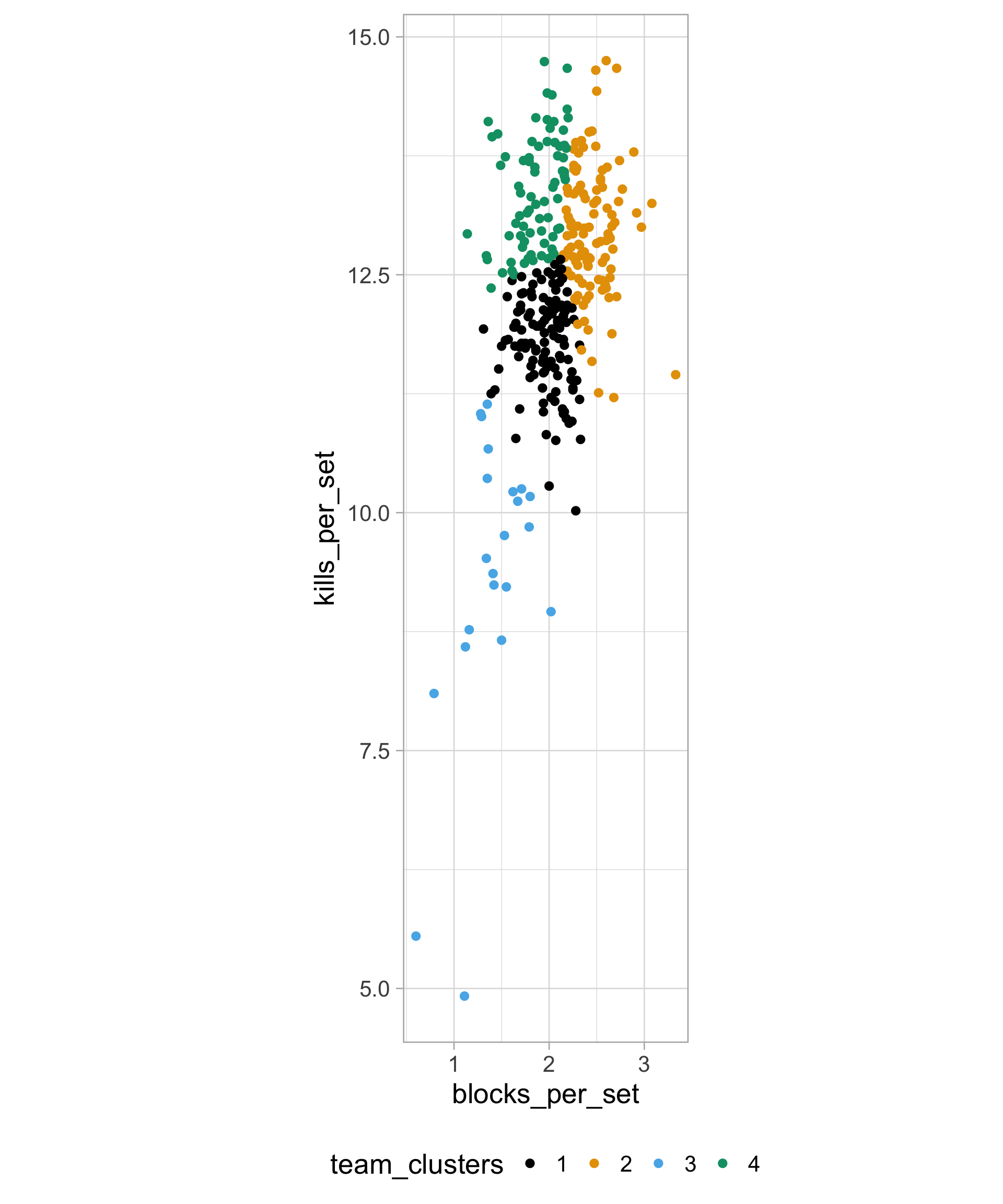
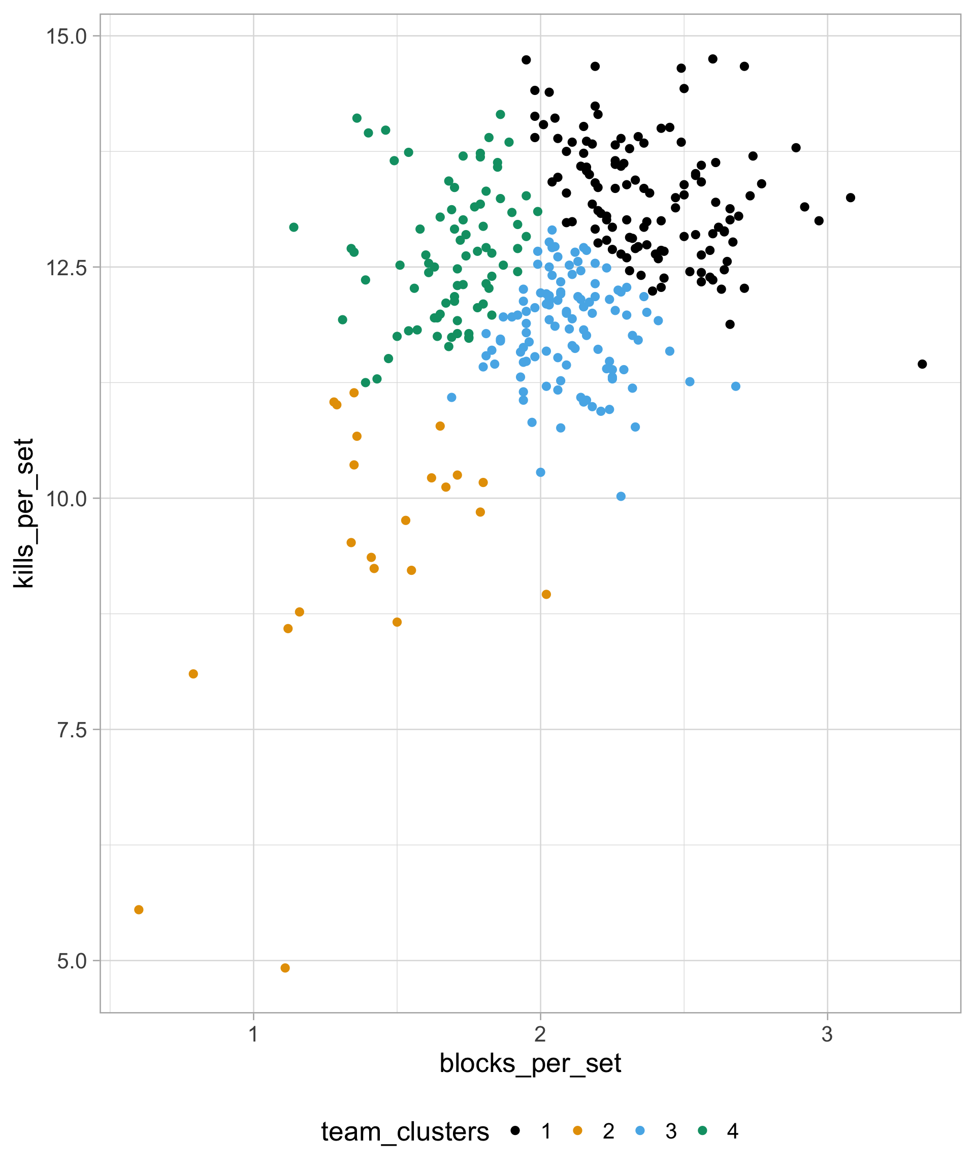
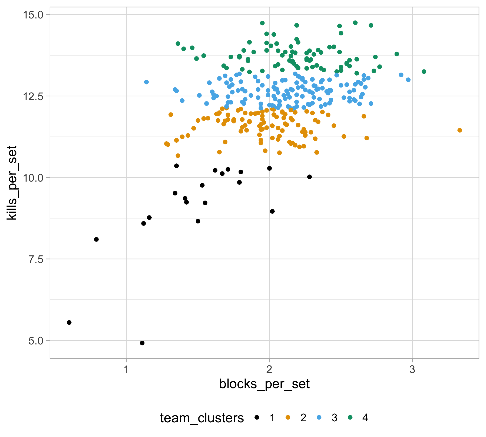
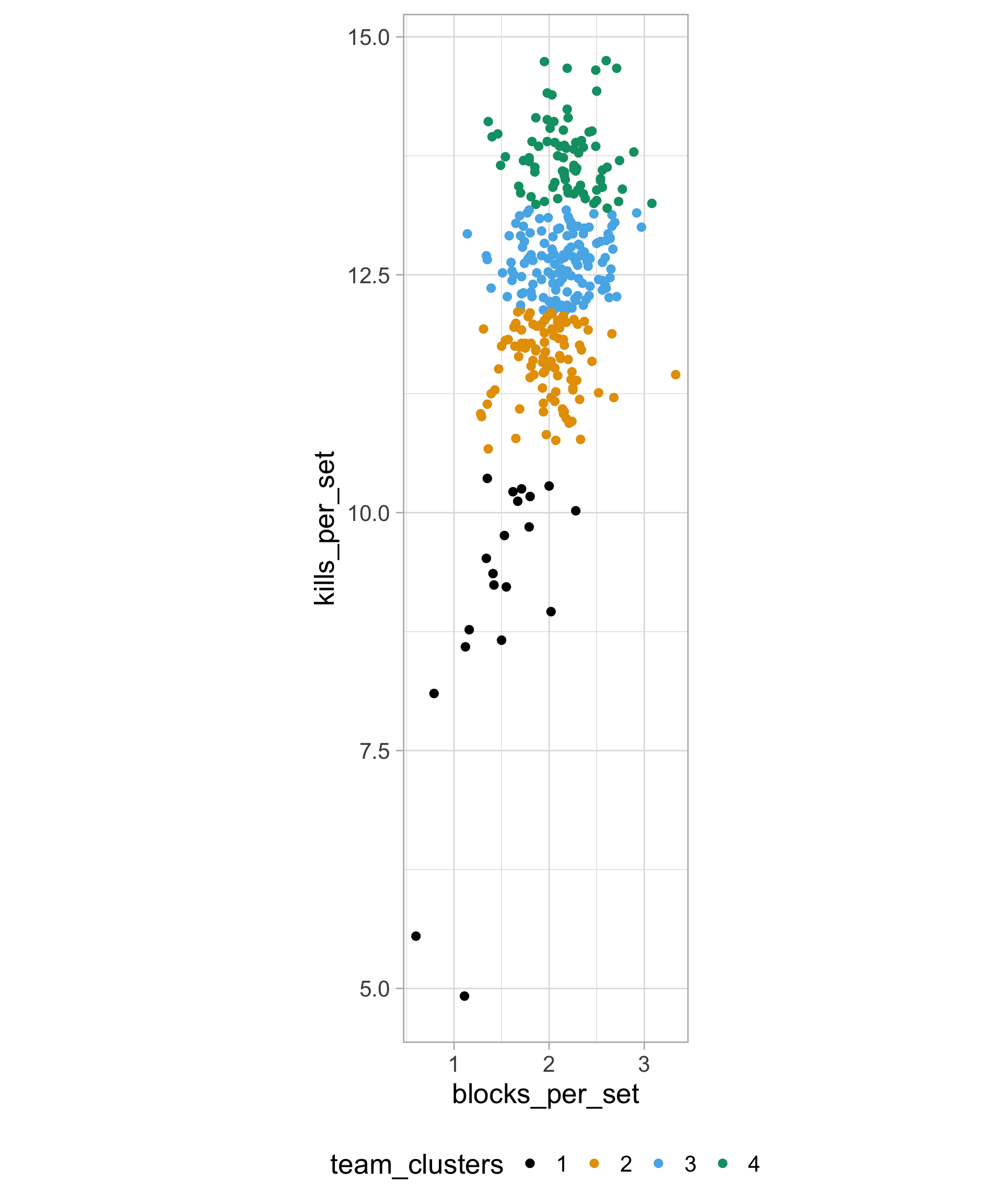
We can do k-means clustering via the kmeans() function in R, but we must provide number of clusters (here we set \(K = 4\))

init_kmeans <- d1_volleyball |> 
  select(kills_per_set, blocks_per_set) |> 
  kmeans(algorithm = "Lloyd", centers = 4,
         nstart = 1, iter.max = 20)

d1_volleyball |>
  mutate(
    team_clusters = as.factor(init_kmeans$cluster)
  ) |>
  ggplot(aes(x = blocks_per_set, y = kills_per_set,
             color = team_clusters)) +
  geom_point(size = 2) + 
  ggthemes::scale_color_colorblind() +
  theme(legend.position = "bottom")

This example only uses 2 features (blocks_per_set and kills_per_set), but in practice, you can (and should) include more than two features

Careful with units…

• We can use coord_fixed() so that the axes match with unit scales

• blocks_per_set and kills_per_set are on very different scales

d1_volleyball |>
  mutate(
    team_clusters = as.factor(init_kmeans$cluster)
  ) |>
  ggplot(aes(x = blocks_per_set, y = kills_per_set, 
             color = team_clusters)) +
  geom_point(size = 2) + 
  ggthemes::scale_color_colorblind() +
  theme(legend.position = "bottom") +
  coord_fixed()

Standardize the variables!

We use the scale() function to first standardize the variables:

\[ \displaystyle \frac{\text{value} - \text{mean}}{\text{standard deviation}} \]

clean_d1_volleyball <- d1_volleyball |>
  mutate(
    std_kills_per_set = as.numeric(scale(kills_per_set, center = TRUE, scale = TRUE)),
    std_blocks_per_set = as.numeric(scale(blocks_per_set, center = TRUE, scale = TRUE))
  )

std_kmeans <- clean_d1_volleyball |> 
  select(std_kills_per_set, std_blocks_per_set) |> 
  kmeans(algorithm = "Lloyd", centers = 4, nstart = 1, iter.max = 20)

clean_d1_volleyball |>
  mutate(
    team_clusters = as.factor(std_kmeans$cluster)
  ) |>
  ggplot(aes(x = blocks_per_set, y = kills_per_set,
             color = team_clusters)) +
  geom_point(size = 2) + 
  ggthemes::scale_color_colorblind() +
  theme(legend.position = "bottom") +
  coord_fixed()

Standardize the variables!

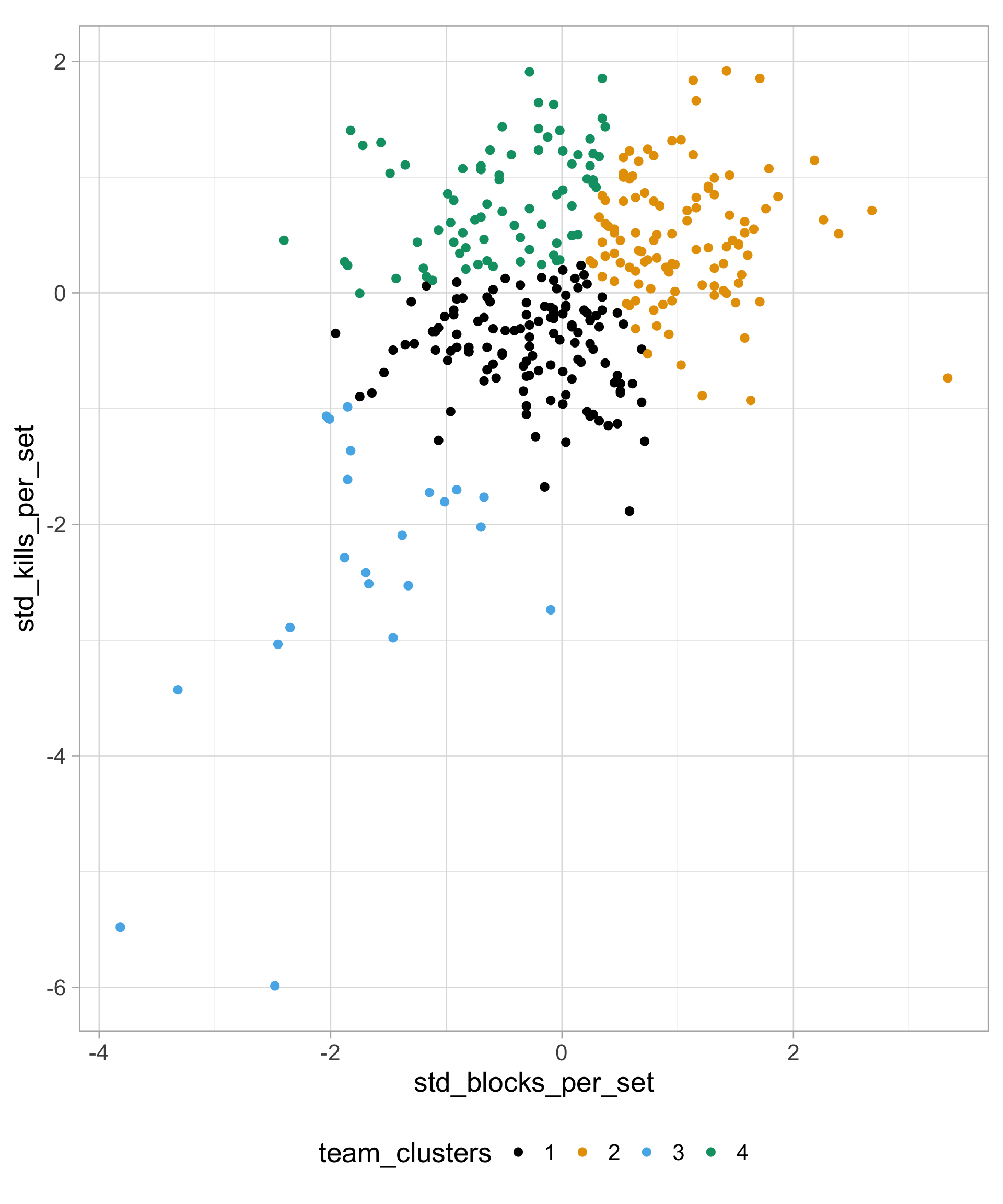
We can also plot the standardized average kills per set and standardized blocks per set

clean_d1_volleyball |>
  mutate(
    team_clusters = as.factor(std_kmeans$cluster)
  ) |>
  ggplot(aes(x = std_blocks_per_set, y = std_kills_per_set,
             color = team_clusters)) +
  geom_point(size = 2) + 
  ggthemes::scale_color_colorblind() +
  theme(legend.position = "bottom") +
  coord_fixed()

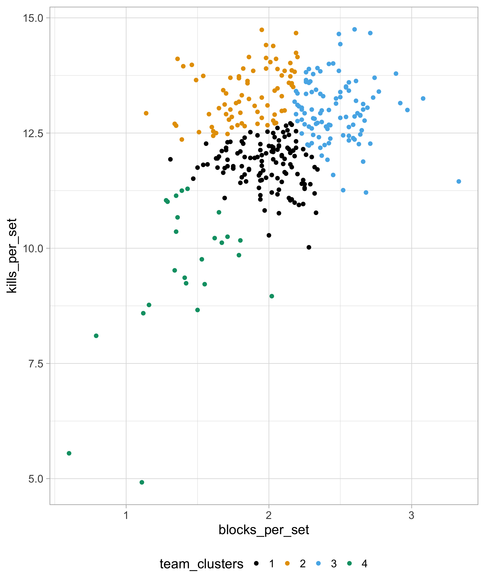
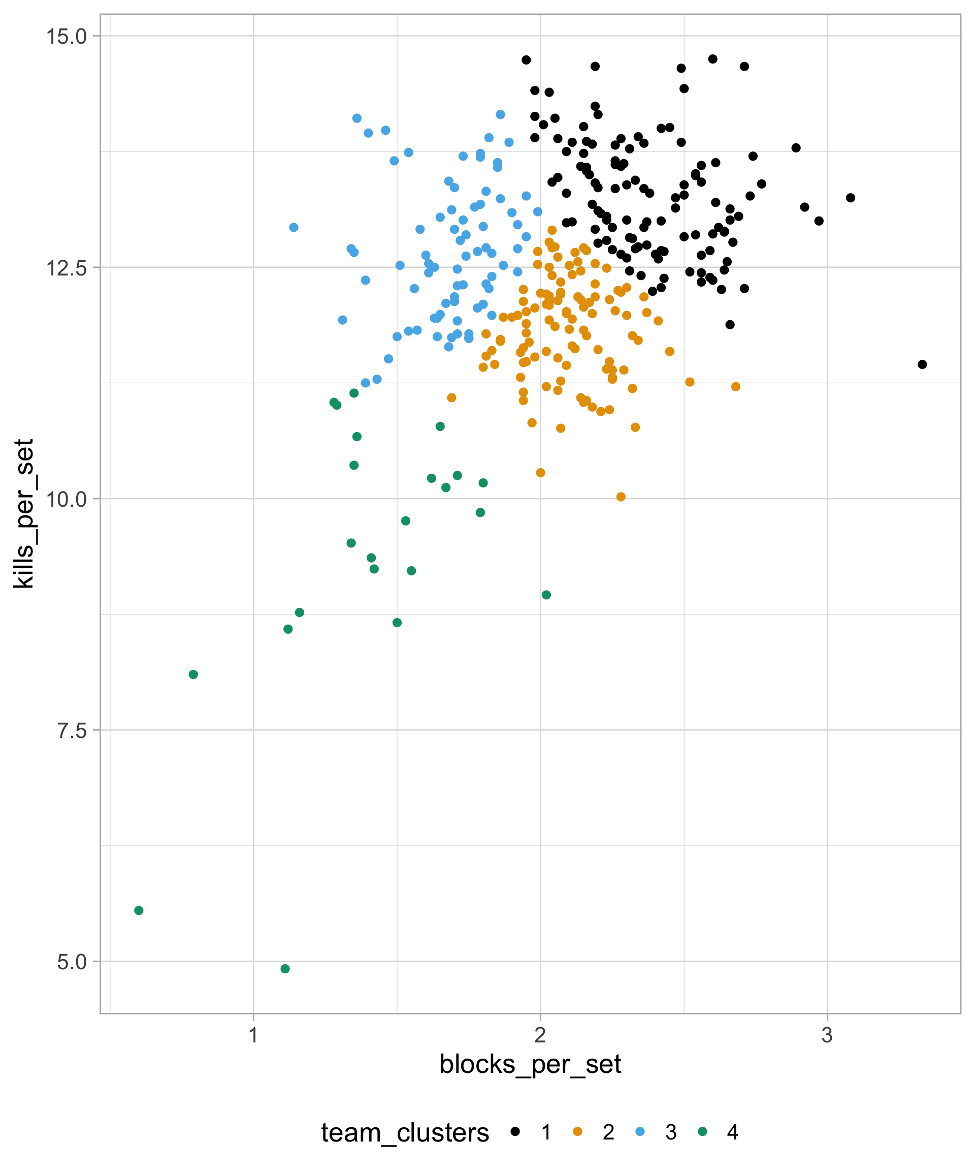
And if we run \(k\)-means again?

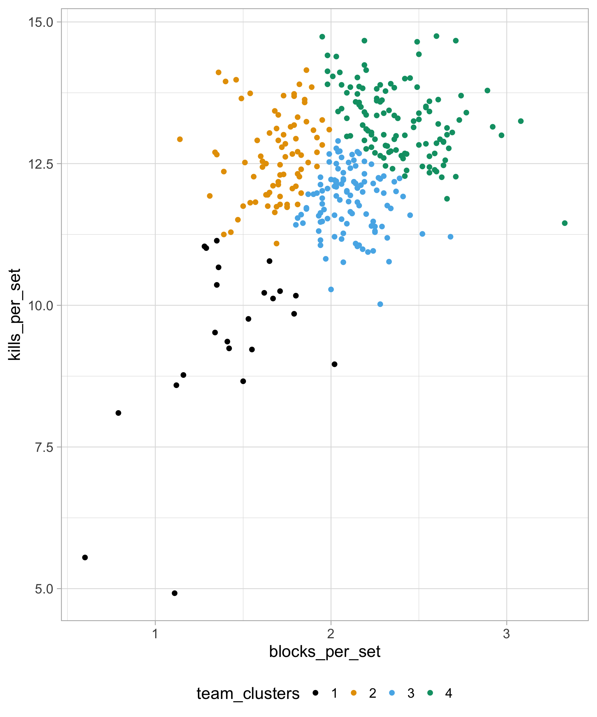
We get different clustering results!

another_kmeans <- clean_d1_volleyball |> 
  select(std_kills_per_set, std_blocks_per_set) |> 
  kmeans(algorithm = "Lloyd", centers = 4, nstart = 1)

clean_d1_volleyball |>
  mutate(
    team_clusters = as.factor(another_kmeans$cluster)
  ) |>
  ggplot(aes(x = blocks_per_set, y = kills_per_set,
             color = team_clusters)) +
  geom_point(size = 2) + 
  ggthemes::scale_color_colorblind() +
  theme(legend.position = "bottom")

Results depend on initial centroids

Keep in mind: the labels / colors are arbitrary

Fix randomness issue with nstart

Run the algorithm nstart times, then pick the results with lowest total within-cluster variation: \[\text{total WSS} = \sum_{k=1}^K W(C_k)\]

nstart_kmeans <- clean_d1_volleyball |> 
  select(std_blocks_per_set, std_kills_per_set) |> 
  kmeans(algorithm = "Lloyd", centers = 4,
         nstart = 30, iter.max = 20)

clean_d1_volleyball |>
  mutate(
    team_clusters = as.factor(nstart_kmeans$cluster)
  ) |> 
  ggplot(aes(x = blocks_per_set, y = kills_per_set,
             color = team_clusters)) +
  geom_point(size = 2) + 
  ggthemes::scale_color_colorblind() +
  theme(legend.position = "bottom")

By default R uses Hartigan–Wong method

• Updates based on changing the cluster assignment of a single observation

• Computational advantages over re-computing distances for every observation

default_kmeans <- clean_d1_volleyball |> 
  select(std_blocks_per_set, std_kills_per_set) |> 
  kmeans(algorithm = "Hartigan-Wong", centers = 4,
         nstart = 30, iter.max = 20) 

clean_d1_volleyball |>
  mutate(
    team_clusters = as.factor(default_kmeans$cluster)
  ) |> 
  ggplot(aes(x = blocks_per_set, y = kills_per_set,
             color = team_clusters)) +
  geom_point(size = 2) + 
  ggthemes::scale_color_colorblind() +
  theme(legend.position = "bottom")

Very little difference for our purposes…

Clustering with more than 2 variables

1. First, we select the variables

d1_volleyball_features <- d1_volleyball |>
  select(blocks_per_set, digs_per_set, kills_per_set, aces_per_set) |> 
  drop_na() 

2. Next, standardize the variables (as always)

std_d1_volleyball_features <- d1_volleyball_features |> 
  scale(center = TRUE, scale = TRUE)

3. Now, perform clustering

kmeans_many_features <- std_d1_volleyball_features |> 
  kmeans(algorithm = "Hartigan-Wong", centers = 4, nstart = 30) 

Clustering with more than 2 variables

One way to examine the clusters is by looking at the (non-standardized) means for each variable included in the cluster analysis

library(gt)

clean_d1_volleyball |>
  select(blocks_per_set, digs_per_set, kills_per_set, aces_per_set) |> 
  mutate(team_clusters = as.factor(kmeans_many_features$cluster)) |> 
  pivot_longer(-team_clusters, names_to = "feature", values_to = "value") |>
  group_by(team_clusters, feature) |>
  summarize(avg_value = mean(value), n_teams = n(), .groups = "drop") |>
  pivot_wider(id_cols = c(team_clusters, n_teams), names_from = feature, values_from = avg_value) |>
  gt() |>
  fmt_number(columns = -n_teams, decimals = 2)

team_clusters	n_teams	aces_per_set	blocks_per_set	digs_per_set	kills_per_set
1	109	1.49	2.38	13.67	12.91
2	42	1.34	1.64	12.85	10.21
3	105	1.29	2.03	15.66	12.50
4	78	1.73	1.86	14.35	12.58

We can also do more EDA: e.g., do teams in the same conference tend be in the same cluster? How does cluster membership relate to win/loss percentage?

Beyond \(k\)-means: \(k\)-means++

Goal: initialize the cluster centers before proceeding with the standard \(k\)-means clustering algorithm, and provide a better alternative to nstart

At a high-level:

• Randomly select an observation to be the first cluster center

• Each subsequent cluster center is chosen from the remaining observations

  • The probability that an observation chosen as a cluster center is proportional to its squared distance from the closest existing cluster center

Visualization of \(k\)-means++

The \(k\)-means++ algorithm

1. Pick a random observation to be the center \(c_1\) of the first cluster \(C_1\)

   • This initializes a set of centers \(\mathscr C = \{c_1 \}\)

2. For each observation (that is not a center), compute \(D(x_i) = \underset{c \in \mathscr C}{\text{min}} \ d(x_i, c)\)

   • Distance between observation and its closest center \(c \in \mathscr C\)

3. Randomly pick a point \(x_i\) with probability: \(\displaystyle p_i = \frac{D^2(x_i)}{\sum_{j=1}^n D^2(x_j)}\)

   • As distance to closest center increases, the probability of selection increases

4. Update \(\mathscr C = \mathscr C \cup c^*\)

5. Repeat steps 3 and 4 until there are \(K\) centers

6. Run \(k\)-means using these \(\mathscr C\) as the starting points

\(k\)-means++ in R using flexclust

library(flexclust)
init_kmeanspp <- clean_d1_volleyball |> 
  select(std_blocks_per_set, std_kills_per_set) |> 
  kcca(k = 4, control = list(initcent = "kmeanspp"))

clean_d1_volleyball |>
  mutate(
    team_clusters = as.factor(init_kmeanspp@cluster)
  ) |>
  ggplot(aes(x = blocks_per_set, y = kills_per_set,
             color = team_clusters)) +
  geom_point(size = 2) + 
  ggthemes::scale_color_colorblind() +
  theme(legend.position = "bottom")

Note the use of @ instead of $…

So, how do we choose the number of clusters?

There is no universally accepted way to conclude that a particular choice of \(k\) is optimal!

From Cosma Shalizi’s notes

One reason you should be intensely skeptical of clustering results — including your own! — is that there is currently very little theory about how to find the right number of clusters. It’s not even completely clear what “the right number of clusters” means!

Additional reading: Statistical Methods for Machine Learning notes

Popular heuristic: elbow plot (use with caution)

Looks at the total within-cluster variation as a function of the number of clusters

Let’s do this by hand first…

# function to perform clustering for each value of k
d1_volleyball_kmeans <- function(k) {
  
  kmeans_results <- clean_d1_volleyball |>
    select(std_blocks_per_set, std_kills_per_set) |>
    kmeans(centers = k, nstart = 30)
  
  kmeans_out <- tibble(
    clusters = k,
    total_wss = kmeans_results$tot.withinss
  )
  return(kmeans_out)
}

# number of clusters to search over
n_clusters_search <- 2:15

# iterate over each k to compute total wss
kmeans_search <- n_clusters_search |> 
  map(d1_volleyball_kmeans) |> 
  bind_rows()

# plot the results
kmeans_search |> 
  ggplot(aes(x = clusters, y = total_wss)) +
  geom_line() + 
  geom_point(size = 4) +
  scale_x_continuous(breaks = n_clusters_search)

Popular heuristic: elbow plot (use with caution)

• Choose \(k\) where marginal improvements is low at the bend (hence the elbow)

  • Based on the plot, this would somewhere around 5–8 clusters

• This is just a guideline and should not dictate your choice of \(k\)

• Other choices: gap statistic, silhouette

Appendix: elbow method with factoextra

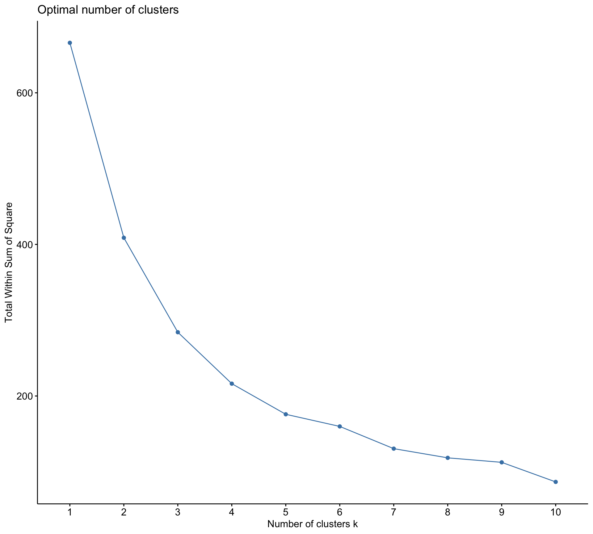
We can also make elbow plots with the factoextra package (also based on total WSS)

library(factoextra)

clean_d1_volleyball |> 
  select(std_blocks_per_set, std_kills_per_set) |> 
  fviz_nbclust(kmeans, method = "wss")

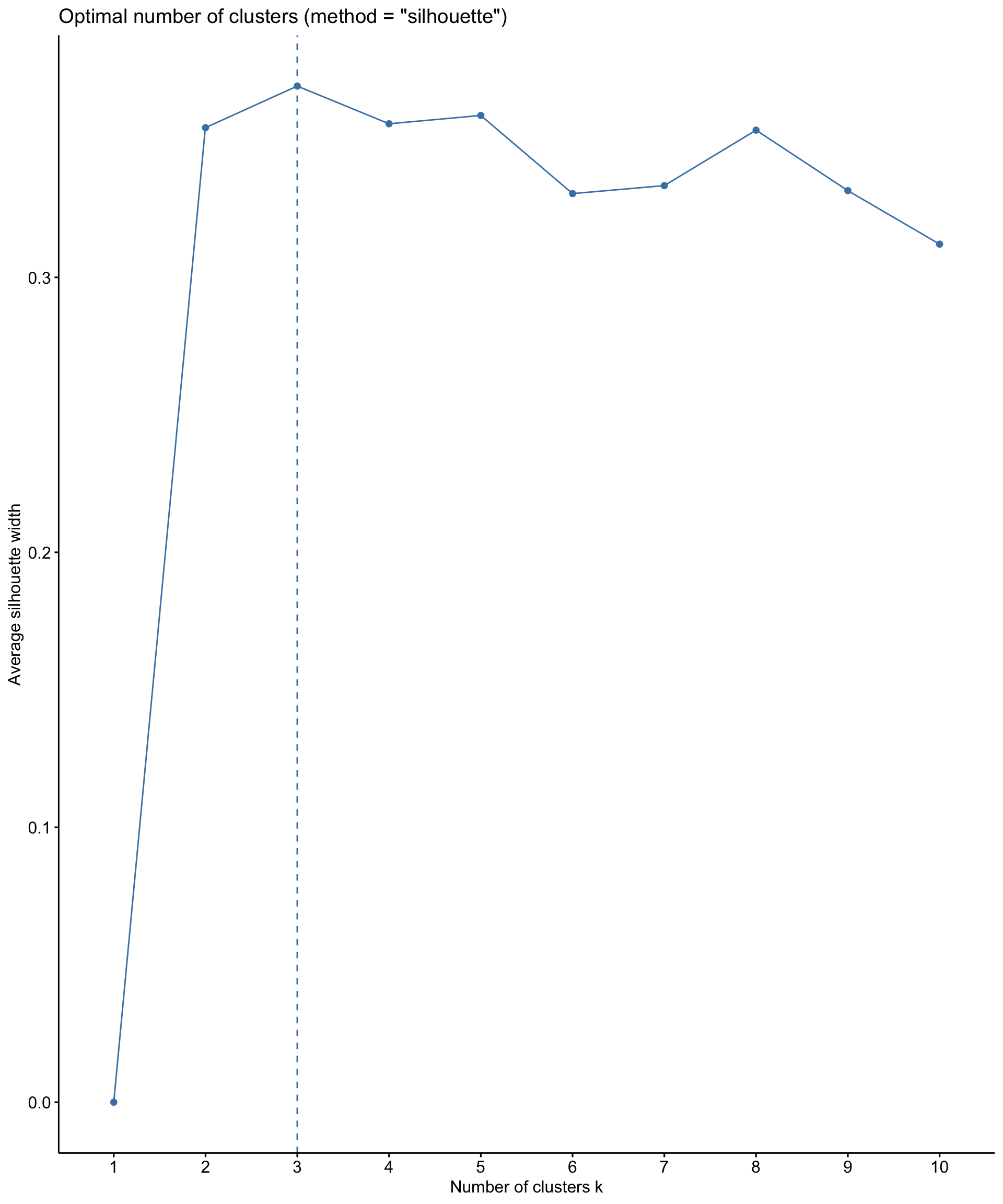
Appendix: silhouette method with factoextra

We can also make a silhouette plot with factoextra

clean_d1_volleyball |> 
  select(std_blocks_per_set, std_kills_per_set) |> 
  fviz_nbclust(kmeans, method = "silhouette")

For more details, see: silhouette (clustering)

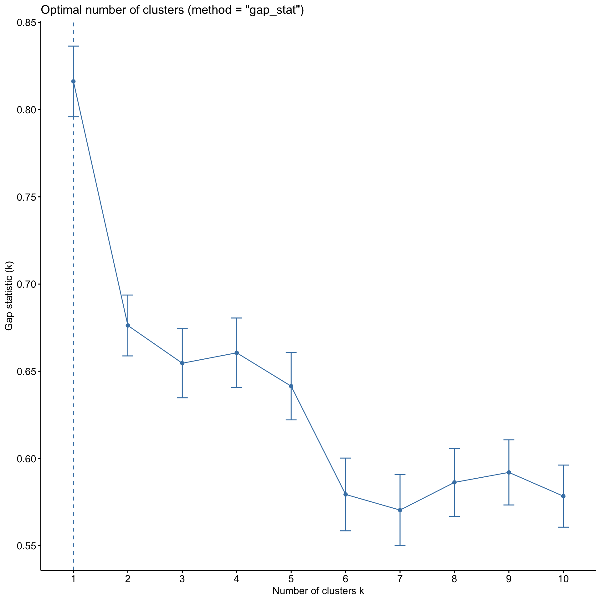
Appendix: gap statistic

We could also compute the gap statistics using the cluster package

library(cluster)

d1_volleyball_kmeans_gap_stat <- clean_d1_volleyball |> 
  select(std_blocks_per_set, std_kills_per_set) |> 
  clusGap(FUN = kmeans, nstart = 30, K.max = 10)

# view the result 
#d1_volleyball_kmeans_gap_stat |> 
#  print(method = "firstmax")

For more details, see: gap statistic

Notice all these methods give a different number of “optimal” clusters!

d1_volleyball_kmeans_gap_stat |> 
  fviz_gap_stat(maxSE = list(method = "firstmax"))

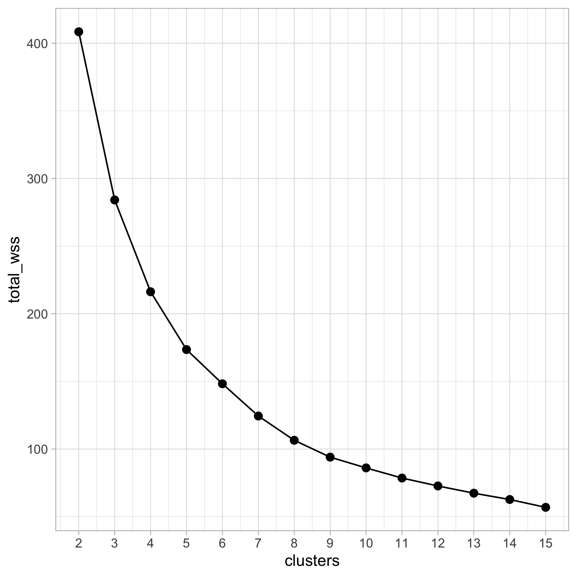
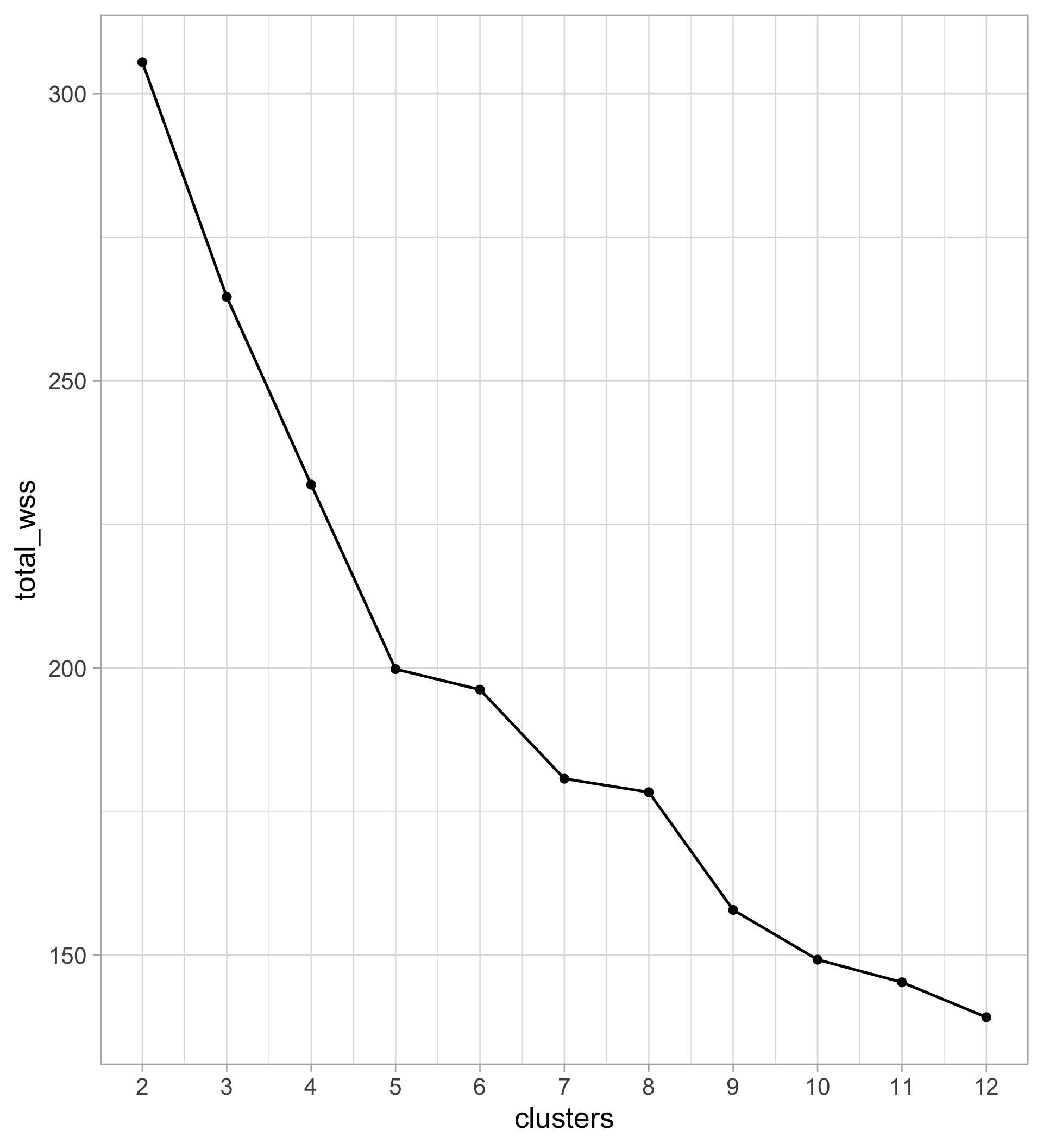
Appendix: elbow plot for \(k\)-means++

d1_volleyball_kmpp <- function(k) {
  
  kmeans_results <- clean_d1_volleyball |>
    select(std_blocks_per_set, std_kills_per_set) |>
    kcca(k = k, control = list(initcent = "kmeanspp"))
  
  kmeans_out <- tibble(
    clusters = k,
    total_wss = sum(kmeans_results@clusinfo$size * 
                      kmeans_results@clusinfo$av_dist)
  )
  return(kmeans_out)
}

n_clusters_search <- 2:12

kmpp_search <- n_clusters_search |> 
  map(d1_volleyball_kmpp) |> 
  bind_rows()

kmpp_search |> 
  ggplot(aes(x = clusters, y = total_wss)) +
  geom_line() + 
  geom_point(size = 2) +
  scale_x_continuous(breaks = n_clusters_search)