Supervised learning: regularization

CMSACamp 2026

Department of Statistics & Data Science
Carnegie Mellon University

Background

Shortcomings of linear regression

• Predictability

  • Recall that we can decompose estimation (prediction) error into squared bias and variance

  • Linear regression: high bias, low variance

• Variable selection

  • With a large number of predictors, it can be helpful to identify a subset of relevant features and eliminate uninformative ones

  • Linear regression “freely” assigns a coefficient to each predictor variable

  • Can we have a model fitting procedure that make only a subset of the coefficients large, and others small (or even better, zero)?

The big picture

Regularized/shrinkage/penalized regression

• Involves fitting a model containing all \(p\) predictors

• However, the estimated coefficients are shrunken towards zero relative to the least squares estimates of vanilla linear regression

• This “shrinkage” (also known as regularization) has the effect of reducing variance

• Depending on what type of regularization is performed, some coefficient estimates can be exactly zero

• Thus, regularization methods (e.g. LASSO) can perform variable selection

Recap: linear regression

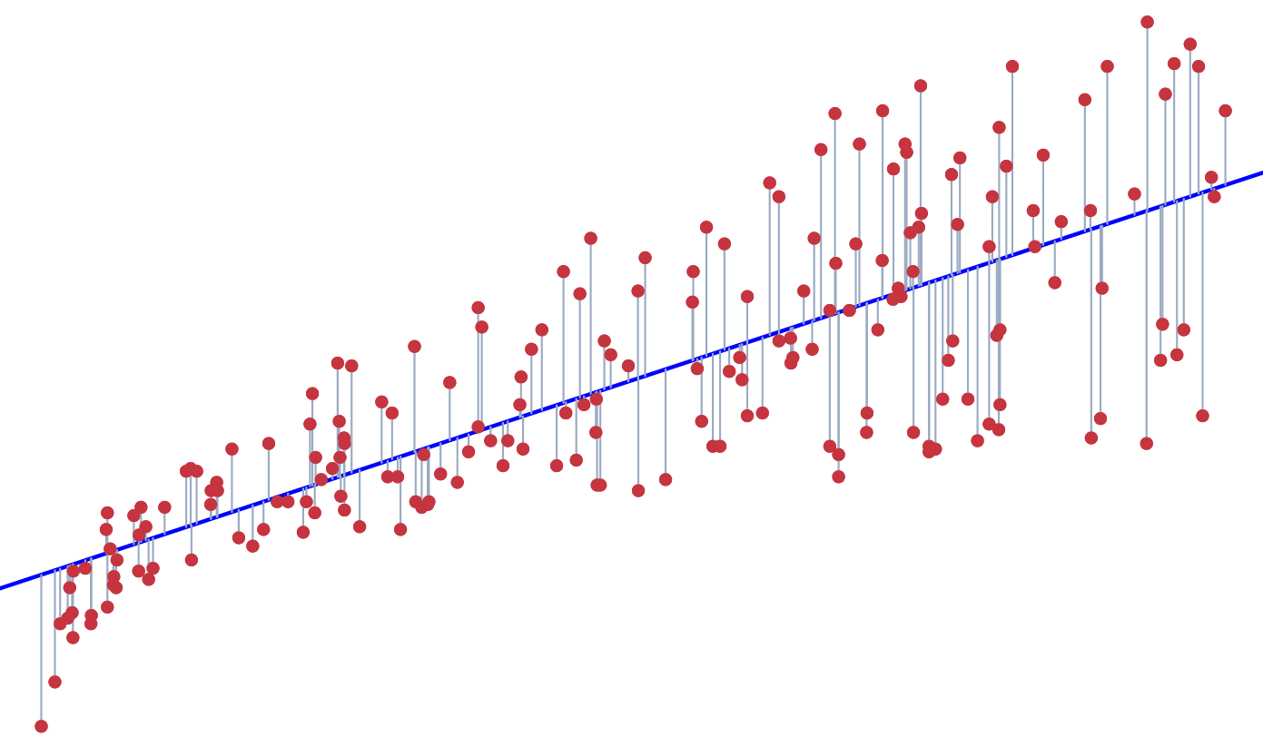
• Linear regression (least squares) estimates coefficients by minimizing

\[\text{RSS} = \sum_{i=1}^n \big(Y_i - \beta_0 - \sum_{j=1}^p \beta_j X_{ij}\big)^2\]

Ridge regression

Linear regression vs ridge regression

• Linear regression (least squares) estimates coefficients by minimizing

\[\text{RSS} = \sum_{i=1}^n \big(Y_i - \beta_0 - \sum_{j=1}^p \beta_j X_{ij}\big)^2\]

• Ridge regression introduces a shrinkage penalty term and minimizes

\[\sum_{i=1}^n \big(Y_i - \beta_0 - \sum_{j=1}^p \beta_j X_{ij}\big)^2 + \lambda \sum_{j=1}^p \beta_j^2 = \text{RSS} + \lambda \sum_{j=1}^p \beta_j^2\]

• Ridge regression uses a (squared) \(\ell_2\) penalty (hence ridge is also known as \(\ell_2\) regularization)

  • The \(\ell_2\) norm of a coefficient vector \(\beta\) is given by \(\displaystyle \Vert \beta \Vert_2 = \sqrt{\sum_{j=1}^p \vert \beta_j \vert ^2}\)

Ridge regression: more details

• Recall that ridge regression minimizes

\[\sum_{i=1}^n \big(Y_i - \beta_0 - \sum_{j=1}^p \beta_j X_{ij}\big)^2 + \lambda \sum_{j=1}^p \beta_j^2 = \text{RSS} + \lambda \sum_{j=1}^p \beta_j^2\]

• Here, \(\lambda \ge 0\) is a tuning parameter, which controls the strength of the penalty term

• Use cross-validation to tune \(\lambda\) (for a fixed value of \(\lambda\), ridge regression fits only a single model)

• As \(\lambda\) increases, flexibility of models decreases (bias increases, variance decreases)

  • When \(\lambda = 0\), it’s just linear regression

  • When \(\lambda \rightarrow \infty\), the coefficient estimates approach 0

  • For \(\lambda\) in between, we are balancing two ideas: fitting a linear model and shrinking the coefficients

Ridge regression: textbook example

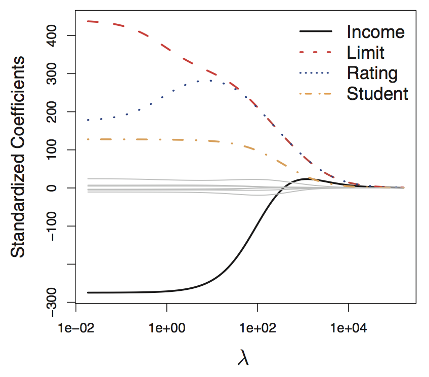
• Notice how the magnitude of the coefficients for the 4 highlighted variables trend as \(\lambda \rightarrow \infty\)

• The coefficients shrink towards zero, but never actually reach it

Lasso & sparsity

Moving from ridge to lasso

• Ridge never sets coefficients to exactly zero (i.e., always keeps all variables)

• Therefore ridge regression cannot perform variable selection

• But we may believe there is a sparse solution (i.e., a model involving only a subset of the variables)

• Entering the lasso (least absolute shrinkage and selection operator)

• Compared to ridge, one big advantage of lasso/sparsity: it performs variable selection in the linear model, so we can understand which relevant features the model relies on for prediction

Linear regression vs ridge vs lasso

• Linear regression (least squares) estimates coefficients by minimizing

\[\text{RSS} = \sum_{i=1}^n \big(Y_i - \beta_0 - \sum_{j=1}^p \beta_j X_{ij}\big)^2\]

• Ridge regression minimizes

\[\sum_{i=1}^n \big(Y_i - \beta_0 - \sum_{j=1}^p \beta_j X_{ij}\big)^2 + \lambda \sum_{j=1}^p \beta_j^2 = \text{RSS} + \lambda \sum_{j=1}^p \beta_j^2\]

• Lasso regression enables variable selection by minimizing

\[\sum_{i=1}^n \big(Y_i - \beta_0 - \sum_{j=1}^p \beta_j X_{ij}\big)^2 + \lambda \sum_{j=1}^p\vert \beta_j \vert = \text{RSS} + \lambda \sum_{j=1}^p \vert \beta_j \vert\]

The lasso: more details

• Recall that the lasso minimizes

\[\sum_{i=1}^n \big(Y_i - \beta_0 - \sum_{j=1}^p \beta_j X_{ij}\big)^2 + \lambda \sum_{j=1}^p\vert \beta_j \vert = \text{RSS} + \lambda \sum_{j=1}^p \vert \beta_j \vert\]

• Lasso uses an \(\ell_1\) penalty (hence also known as \(\ell_1\) regularization)

  • The \(\ell_1\) norm of a coefficient vector \(\beta\) is given by \(\displaystyle \Vert \beta \Vert_1 = \sum_{j=1}^p \vert \beta_j \vert\)

• The only difference between lasso and ridge is that ridge uses a (squared) \(\ell_2\) penalty \(\Vert \beta \Vert_2^2\), while lasso uses an \(\vert \ell_1 \vert\) penalty

• Importantly, although these two problems look relatively similar, their solutions behave very differently

The lasso: more details

• Recall that the lasso minimizes

\[\sum_{i=1}^n \big(Y_i - \beta_0 - \sum_{j=1}^p \beta_j X_{ij}\big)^2 + \lambda \sum_{j=1}^p\vert \beta_j \vert = \text{RSS} + \lambda \sum_{j=1}^p \vert \beta_j \vert\]

• Here, \(\lambda \ge 0\) is a tuning parameter, which controls the strength of the penalty (like ridge)

• Use cross-validation to tune \(\lambda\) (for a fixed value of \(\lambda\), lasso regression fits only a single model)

• As \(\lambda\) increases, flexibility of models decreases (bias increases, variance decreases)

  • When \(\lambda = 0\), it’s just linear regression

  • When \(\lambda \rightarrow \infty\), the coefficient estimates approach 0

  • For \(\lambda\) in between, we are balancing two ideas: fitting a linear model and shrinking the coefficients

  • But the nature of the \(\ell_1\) penalty allows some coefficients to be shrunken to zero exactly

• Lasso can handle the \(p > n\) case, i.e. more variables than observations

Shrinkage methods: lasso regression

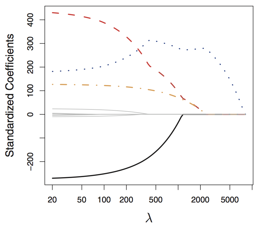
• Lasso regression performs variable selection yielding sparse models (i.e. models that involve only a subset of the variables)

• We get different models with different number of predictors at different values of \(\lambda\)

• The coefficients shrink towards and eventually equal zero

Why doesn’t ridge set coefficients equal to 0?

• Ridge minimizes \(\text{RSS} + \lambda \sum_{j=1}^p \beta_j^2\)

• Taking the derivative of the objective function: \(\frac{d}{d\beta_j}(\text{RSS} + \lambda \sum_{j=1}^p \beta_j^2) = \frac{d\text{RSS}}{d\beta_j} + 2\lambda \beta_j\)

• Near zero: As \(\beta_j \rightarrow 0\), \(2\lambda \beta_j \rightarrow 0\), so the penalty exerts almost no force near zero.

• Idea: The penalty pulls coefficients toward zero, but the pull becomes weaker as coefficients get smaller, so coefficients are rarely exactly zero.

Why does lasso set coeffcients equal to 0?

• LASSO minimizes \(\text{RSS} + \lambda \sum_{j=1}^p \vert \beta_j \vert\)

• Taking the derivative of the objective function: \(\frac{d}{d\beta_j}(\text{RSS} + \lambda \sum_{j=1}^p |\beta_j|) = \frac{d\text{RSS}}{d\beta_j} + \lambda \text{sign}(\beta_j)\)

• The derivative (think of it as how strong the penalty pull is) stays the same no matter how close \(\beta_j\) gets to 0.

• The consequence is that if \(\Big| \frac{d \text{RSS}}{d\beta_j} \Big| < \lambda\), the improvement in fit is too small to overcome the penalty, and the optimal solution is \(\beta_j = 0\).

• Idea: Lasso applies a constant pull toward zero. Variables with only a weak contribution to model fit are pulled all the way to exactly zero.

Elastic net

Best of both worlds: elastic net

• Motivation: when developing models, there are often strong correlations among the features

• The lasso penalty is somewhat indifferent to the choice among a set of strong but correlated features

• The ridge penalty tends to shrink the coefficients of correlated features toward each other

• The elastic net penalty is a compromise, aiming to

  • encourages highly correlated features to be average

  • encourages a sparse solution in the coefficients of these averaged features

• From the original paper’s abtract:

… the elastic net encourages a grouping effect, where strongly correlated predictors tend to be in or out of the model together.

Ridge vs lasso vs elastic net

• Ridge minimizes

\[\sum_{i=1}^n \big(Y_i - \beta_0 - \sum_{j=1}^p \beta_j X_{ij}\big)^2 + \lambda \sum_{j=1}^p \beta_j^2 = \text{RSS} + \lambda \sum_{j=1}^p \beta_j^2\]

• Lasso minimizes

\[\sum_{i=1}^n \big(Y_i - \beta_0 - \sum_{j=1}^p \beta_j X_{ij}\big)^2 + \lambda \sum_{j=1}^p\vert \beta_j \vert = \text{RSS} + \lambda \sum_{j=1}^p \vert \beta_j \vert\]

• Elastic net compromises between ridge and lasso

\[\sum_{i=1}^{n}\left(Y_{i}-\beta_{0}-\sum_{j=1}^{p} \beta_{j} X_{i j}\right)^{2}+\lambda\left(\frac{1-\alpha}{2}\|\beta\|_{2}^{2}+\alpha\|\beta\|_{1} \right)\]

Elastic net: more details

• Elastic net minimizes

\[\sum_{i=1}^{n}\left(Y_{i}-\beta_{0}-\sum_{j=1}^{p} \beta_{j} X_{i j}\right)^{2}+\lambda\left(\frac{1-\alpha}{2}\|\beta\|_{2}^{2}+\alpha\|\beta\|_{1} \right)\]

• Penalty terms: \(\lambda \cdot (1 - \alpha) / 2\) (ridge) and \(\lambda \cdot \alpha\) (lasso)

  • \(\alpha\) controls the mixing between the two types, ranges from 0 to 1

  • \(\alpha = 1\) returns lasso, \(\alpha = 0\) return ridge

• \(\lambda\) and \(\alpha\) are tuning parameters; use cross-validation to tune

Scaling of predictors

• In linear regression, the (least squares) coefficient estimates are scale equivariant

  • Multiplying \(X_j\) by a constant c simply leads to a scaling of the least squares coefficient estimates by a factor of \(1/c\)

  • i.e., regardless of how the \(j\)th predictor is scaled, \(X_j \hat \beta_j\) will remain the same

• For ridge, lasso, and elastic net: standardize the predictors

  • The coefficient estimates can change substantially when multiplying a given predictor by a constant, due to the sum of squared coefficients term in the penalty

  • For each predictor column, subtract off the mean, and divide by the standard deviation \[\tilde{x}_{ij} = \frac{x_{ij} - \bar{x}_j}{s_{x,j}}\]

Data: NFL teams summary

Dataset summarizes NFL team performances from 1999 to 2021

library(tidyverse)
theme_set(theme_light())

nfl_teams_data <- read_csv("http://www.stat.cmu.edu/cmsac/sure/2022/materials/data/sports/regression_examples/nfl_team_season_summary.csv")
nfl_model_data <- nfl_teams_data %>%
  mutate(score_diff = points_scored - points_allowed) %>%
  filter(season >= 2006) %>% # Only use rows with air yards
  dplyr::select(-wins, -losses, -ties, -points_scored, -points_allowed, -season, -team)

Introduction to glmnet

Fit ridge, lasso, and elastic net models with glmnet. To start, create predictor matrix and response vector:

library(glmnet)

# predictors
model_x <- nfl_model_data |> 
  dplyr::select(-score_diff) |>
  as.matrix()

# response
model_y <- nfl_model_data |> 
  pull(score_diff)

Vanilla linear regression model

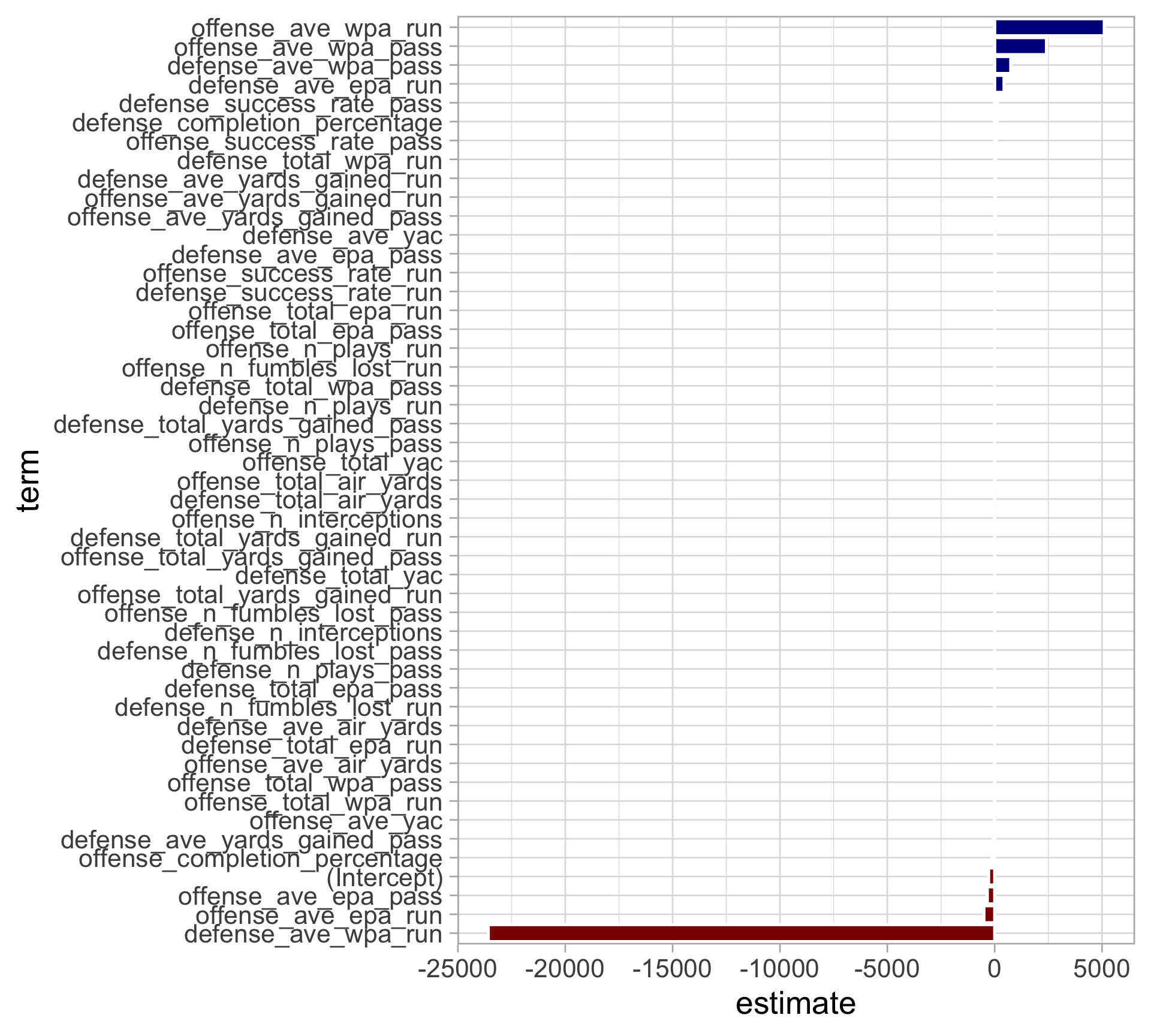
• What do the initial regression coefficients look like?

• Use broom to tidy model output for plotting

init_reg_fit <- lm(score_diff ~ ., data = nfl_model_data)
library(broom)
init_reg_fit |> 
  tidy() |> 
  mutate(term = fct_reorder(term, estimate)) |> 
  ggplot(aes(x = estimate, y = term, 
             fill = estimate > 0)) +
  geom_col(color = "white", show.legend = FALSE) +
  scale_fill_manual(values = c("darkred", "darkblue"))

Ridge regression

Perform ridge regression using glmnet with alpha = 0

By default, predictors are standardized and models are fitted across a range of \(\lambda\) values

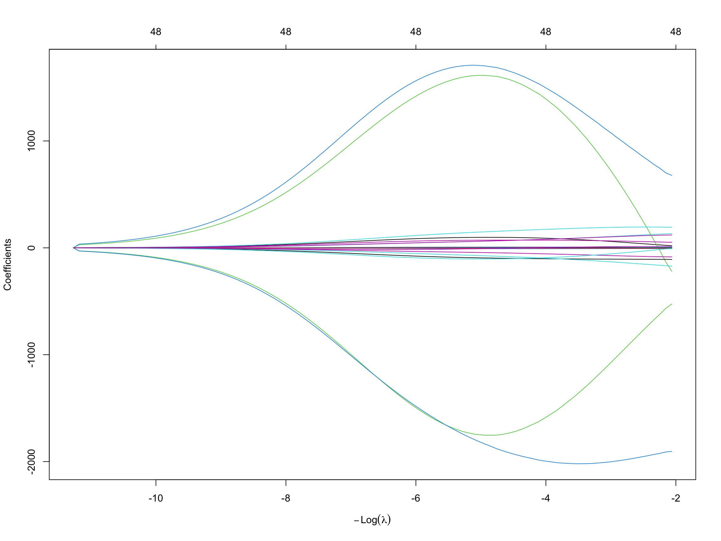
init_ridge_fit <- glmnet(model_x, model_y, alpha = 0)
plot(init_ridge_fit, xvar = "lambda")

Ridge regression

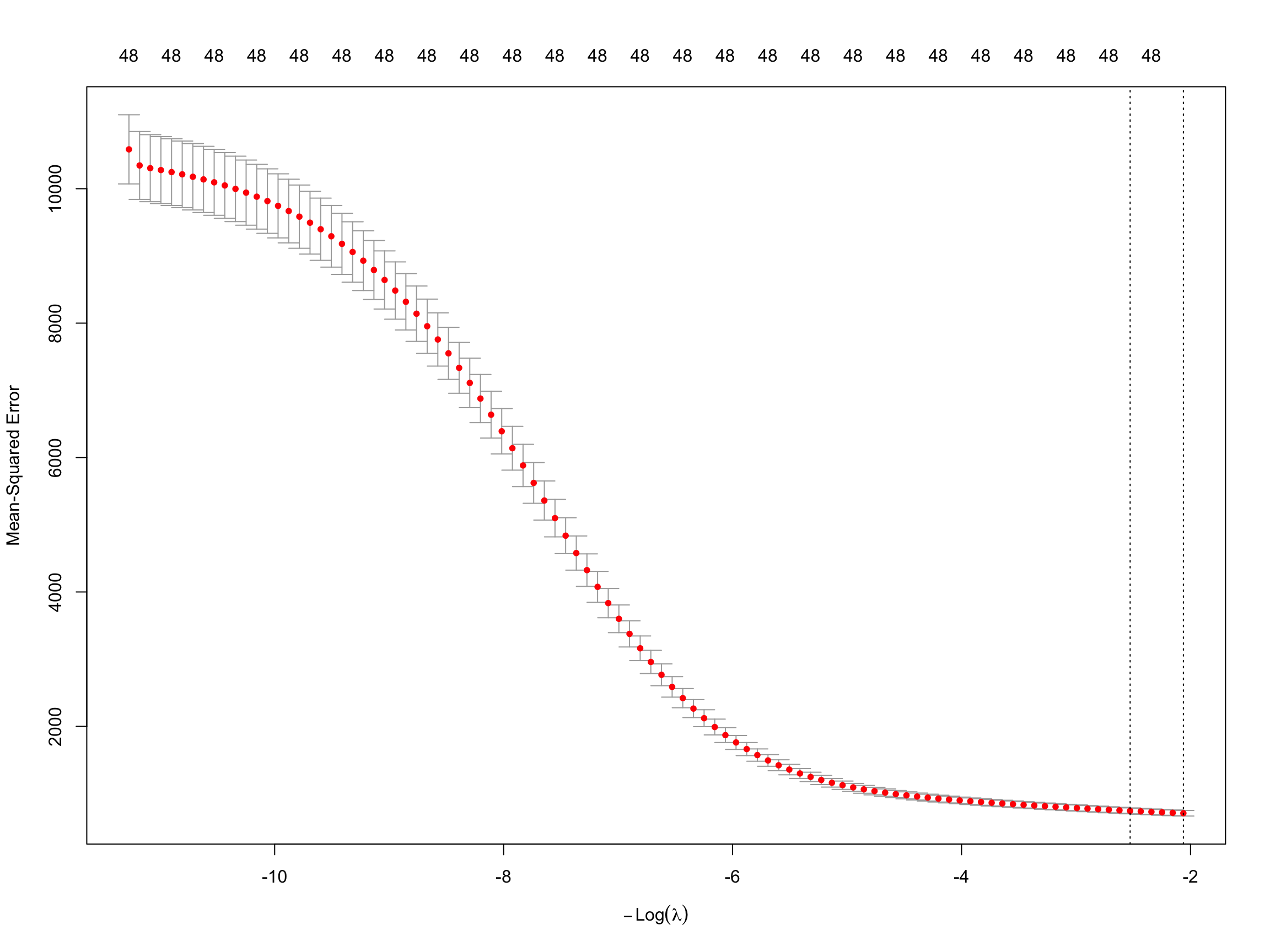
Use cross-validation to select \(\lambda\) with cv.glmnet() which uses 10 folds by default

Specify ridge regression with alpha = 0

fit_ridge_cv <- cv.glmnet(model_x, model_y, alpha = 0)
plot(fit_ridge_cv)

Tidy ridge regression

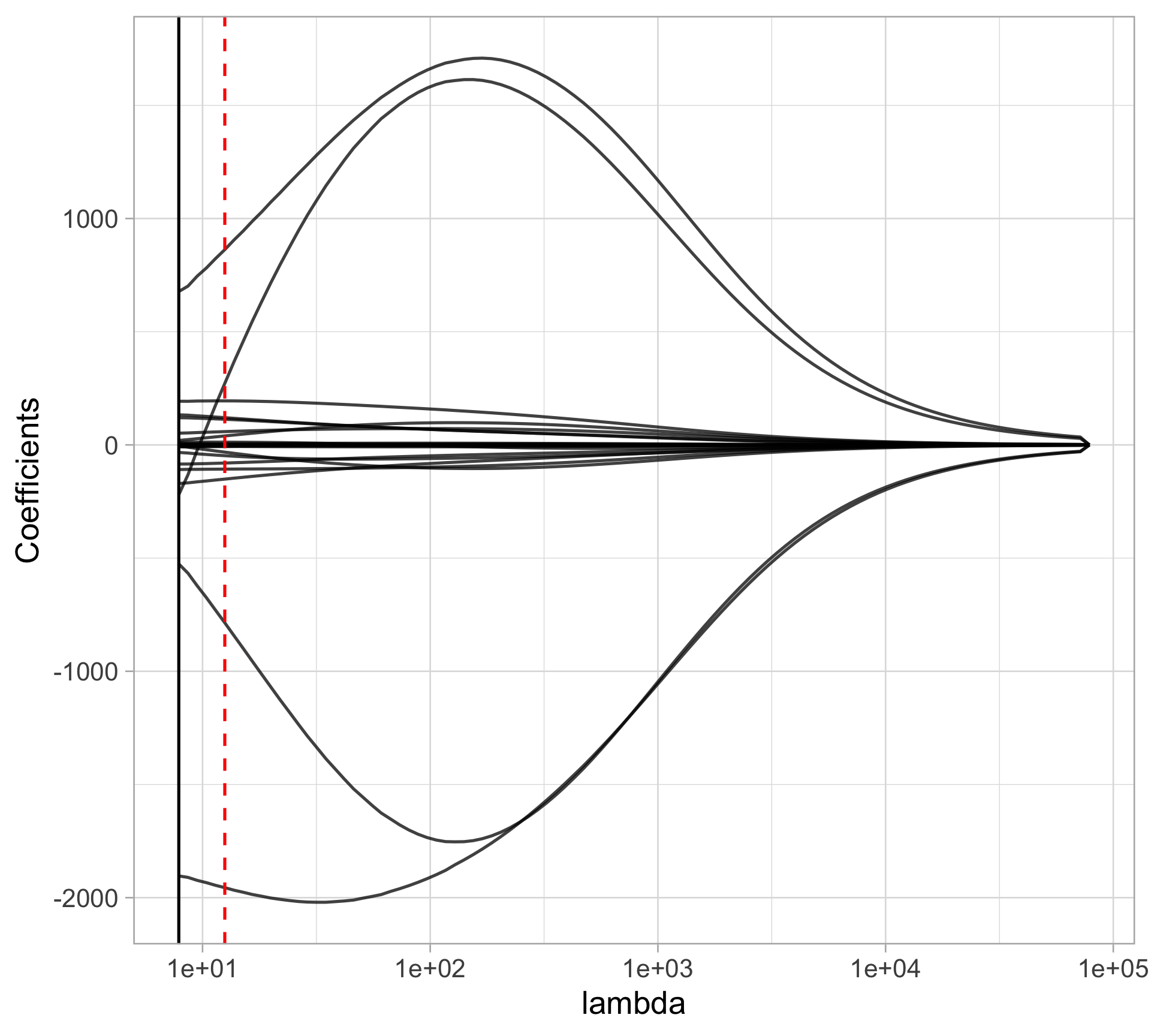
tidy_ridge_coef <- tidy(fit_ridge_cv$glmnet.fit)
tidy_ridge_coef |> 
  ggplot(aes(x = lambda, y = estimate, group = term)) +
  scale_x_log10() +
  geom_line(alpha = 0.75) +
  geom_vline(xintercept = fit_ridge_cv$lambda.min) +
  geom_vline(xintercept = fit_ridge_cv$lambda.1se, 
             linetype = "dashed", color = "red")+
  labs(y = "Coefficients")

Could easily add color with legend for variables…

Tidy ridge regression

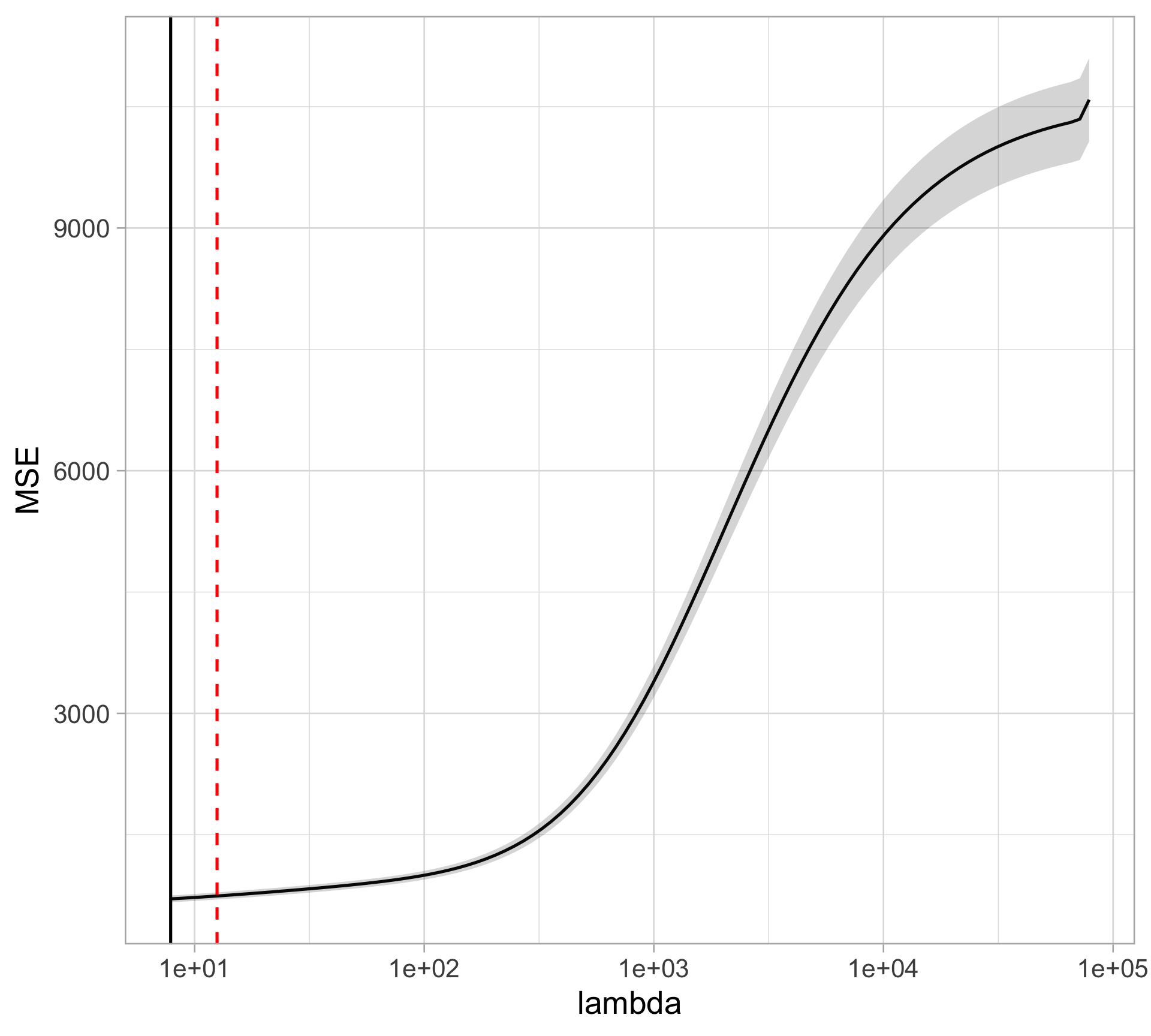
tidy_ridge_cv <- tidy(fit_ridge_cv)
tidy_ridge_cv |> 
  ggplot(aes(x = lambda, y = estimate)) +
  geom_line() + 
  scale_x_log10() +
  geom_ribbon(aes(ymin = conf.low, ymax = conf.high), 
              alpha = 0.2) +
  geom_vline(xintercept = fit_ridge_cv$lambda.min) +
  geom_vline(xintercept = fit_ridge_cv$lambda.1se,
             linetype = "dashed", color = "red")+
   labs(y = "MSE")

Ridge regression coefficients

Coefficients using the one-standard-error rule

(select the model with estimated test error within 1 SE of the minimum test error)

#ridge_final <- glmnet(
#  model_x, model_y, alpha = 0,
#  lambda = fit_ridge_cv$lambda.1se,
#)
#library(vip)
#ridge_final |>
#  vip()

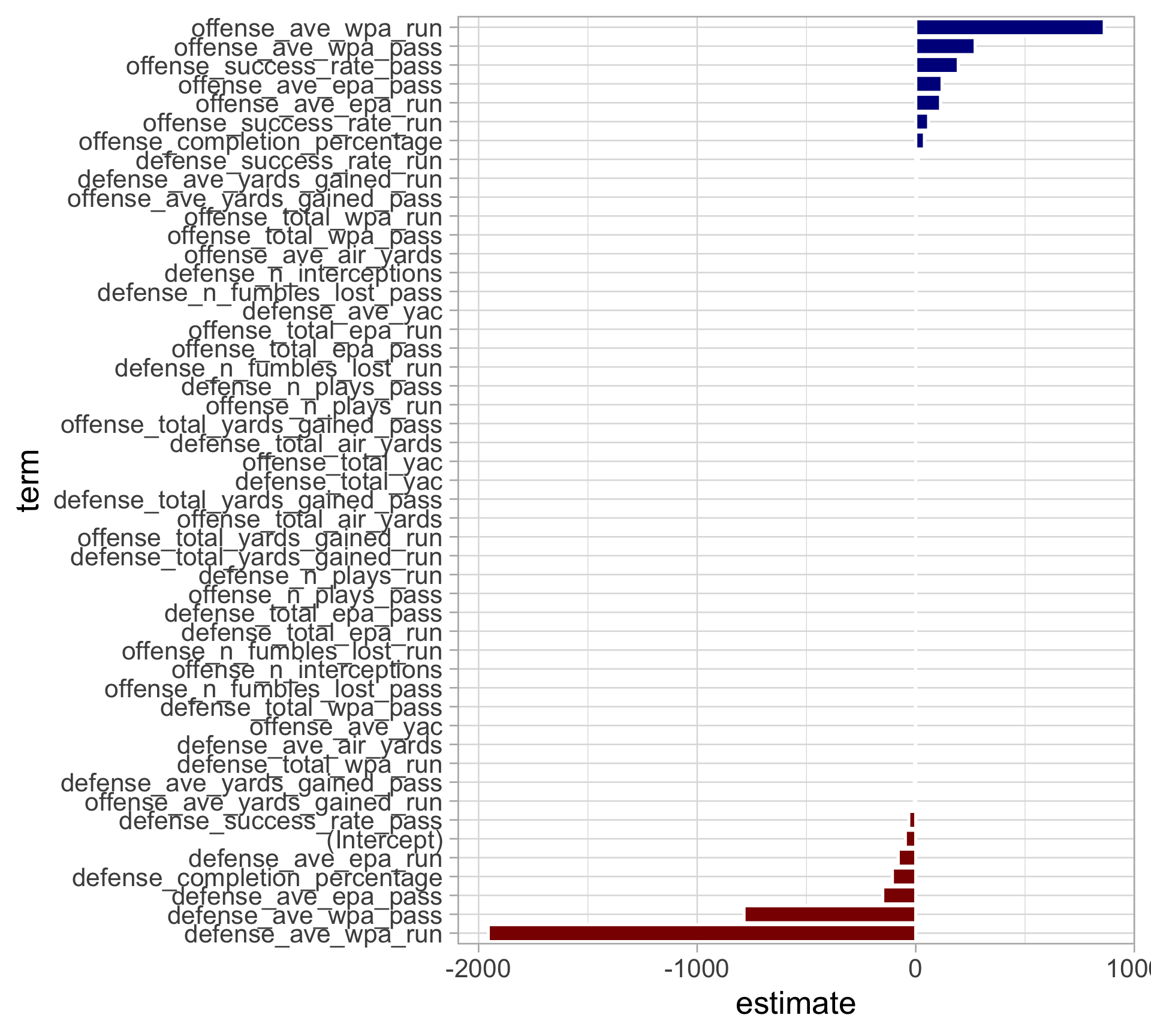
tidy_ridge_coef |>
  filter(lambda == fit_ridge_cv$lambda.1se) |>
  mutate(term = fct_reorder(term, estimate)) |>
  ggplot(aes(x = estimate, y = term, 
             fill = estimate > 0)) +
  geom_col(color = "white", show.legend = FALSE) +
  scale_fill_manual(values = c("darkred", "darkblue"))

Lasso regression example

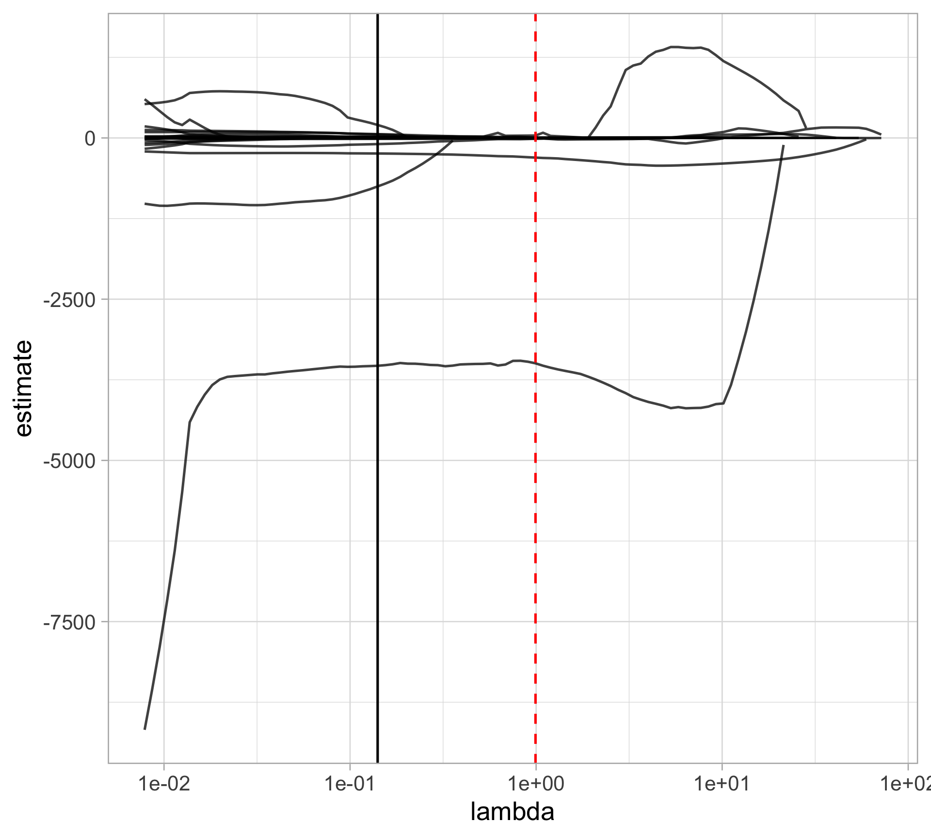
Similar syntax to ridge but specify alpha = 1:

fit_lasso_cv <- cv.glmnet(model_x, model_y, 
                               alpha = 1)
tidy_lasso_coef <- tidy(fit_lasso_cv$glmnet.fit)
tidy_lasso_coef |> 
  ggplot(aes(x = lambda, y = estimate, group = term)) +
  scale_x_log10() +
  geom_line(alpha = 0.75) +
  geom_vline(xintercept = fit_lasso_cv$lambda.min) +
  geom_vline(xintercept = fit_lasso_cv$lambda.1se, 
             linetype = "dashed", color = "red")

Lasso regression example

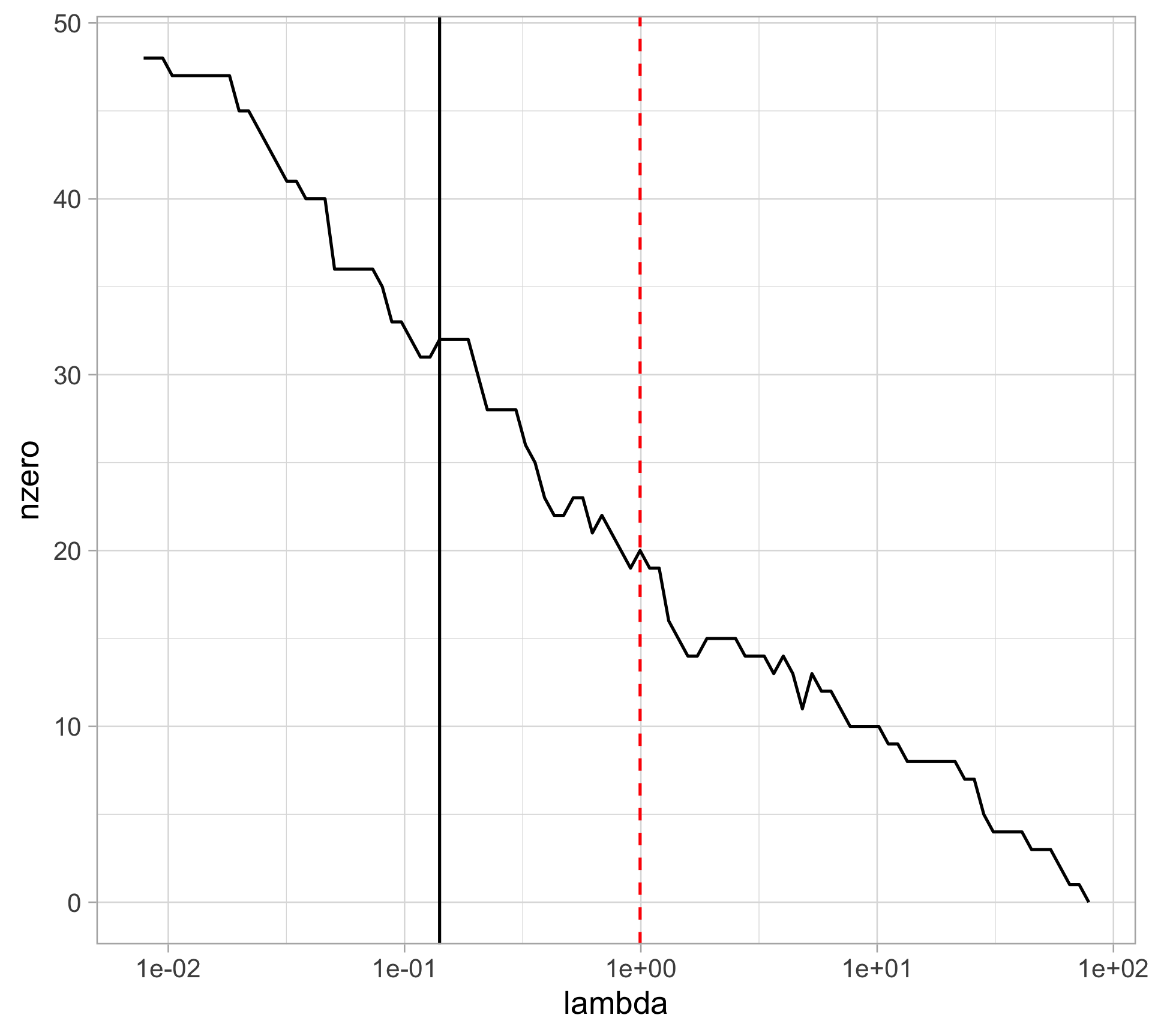
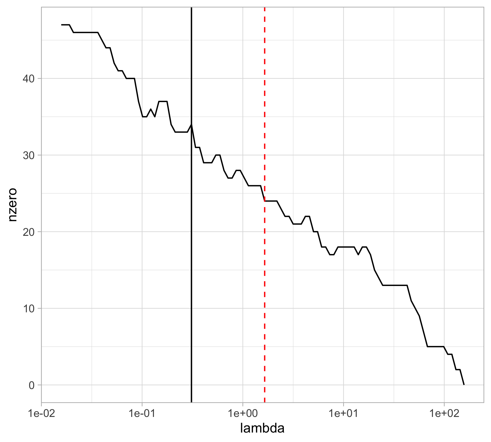
Number of non-zero predictors by \(\lambda\)

tidy_lasso_cv <- tidy(fit_lasso_cv)
tidy_lasso_cv |>
  ggplot(aes(x = lambda, y = nzero)) +
  geom_line() +
  geom_vline(xintercept = fit_lasso_cv$lambda.min) +
  geom_vline(xintercept = fit_lasso_cv$lambda.1se, 
             linetype = "dashed", color = "red") +
  scale_x_log10()

Reduction in variables using one-standard-error rule

Lasso regression example

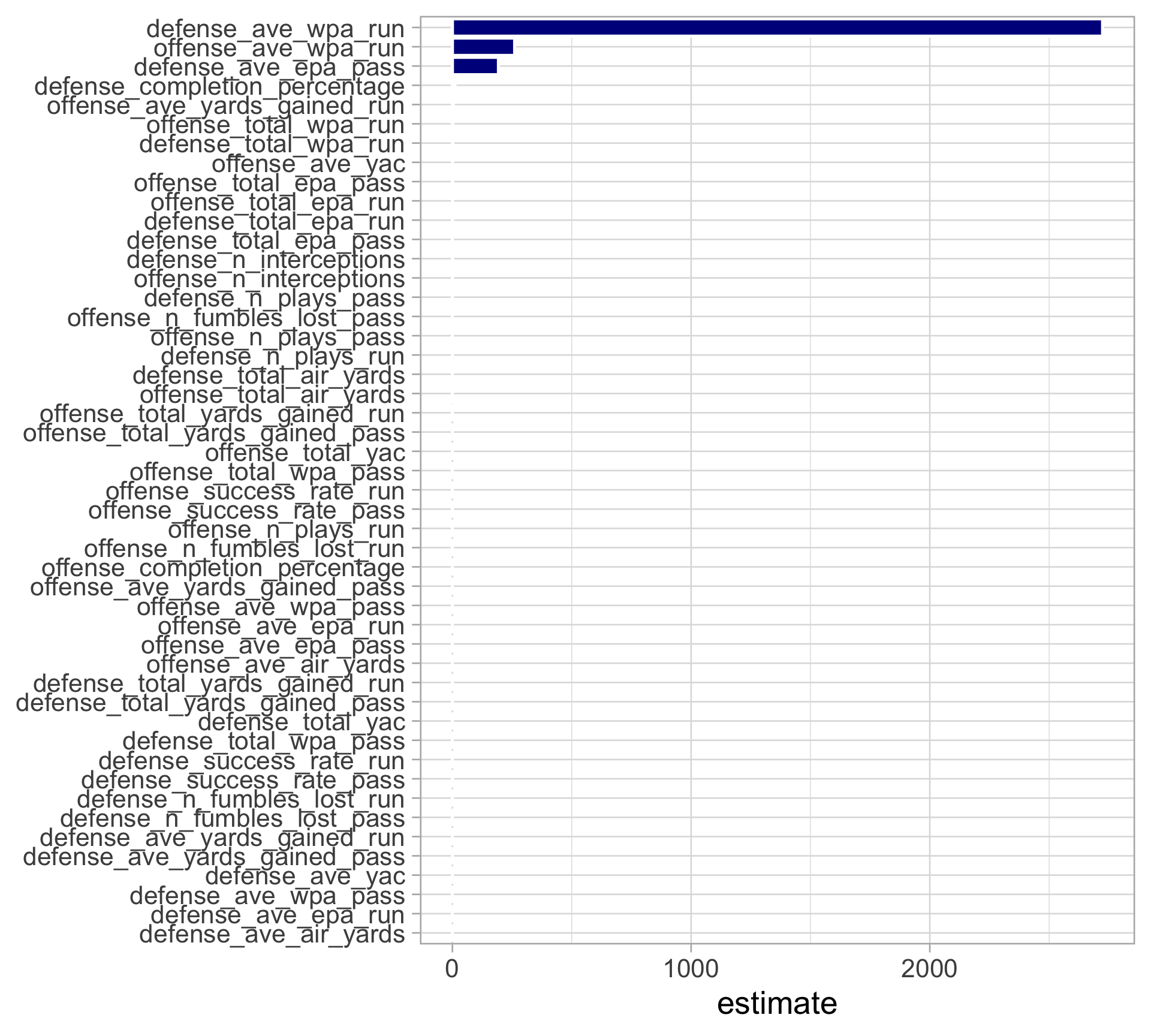
Coefficients using the one-standard-error rule

# this will only print out non-zero coefficient estimates
# tidy_lasso_coef |>
#   filter(lambda == fit_lasso_cv$lambda.1se)

lasso_final <- glmnet(
  model_x, model_y, 
  alpha = 1,
  lambda = fit_lasso_cv$lambda.1se,
)
library(vip)
lasso_final |> 
  vi() |> 
  mutate(Variable = fct_reorder(Variable, Importance)) |>
  ggplot(aes(x = Importance, y = Variable, 
             fill = Importance > 0)) +
  geom_col(color = "white", show.legend = FALSE) +
  scale_fill_manual(values = c("darkred", "darkblue")) +
  labs(x = "estimate", y = NULL)

Elastic net example

Need to tune both \(\lambda\) and \(\alpha\) - can do so manually with our own folds

set.seed(100)
fold_id <- sample(rep(1:10, length.out = nrow(model_x)))

Then use cross-validation with these folds for different candidate alpha values:

cv_enet_25 <- cv.glmnet(model_x, model_y, foldid = fold_id, alpha = 0.25)
cv_enet_50 <- cv.glmnet(model_x, model_y, foldid = fold_id, alpha = 0.5)
cv_ridge <- cv.glmnet(model_x, model_y, foldid = fold_id, alpha = 0)
cv_lasso <- cv.glmnet(model_x, model_y, foldid = fold_id, alpha = 1)

Can see which one had the lowest CV error among its candidate \(\lambda\) values:

which.min(c(min(cv_enet_25$cvm), min(cv_enet_50$cvm), min(cv_ridge$cvm), min(cv_lasso$cvm)))

[1] 4

Elastic net example

Can view same type of summary

cv_enet_50 |> 
  tidy() |> 
  ggplot(aes(x = lambda, y = nzero)) +
  geom_line() +
  geom_vline(xintercept = cv_enet_50$lambda.min) +
  geom_vline(xintercept = cv_enet_50$lambda.1se, 
             linetype = "dashed", 
             color = "red") +
  scale_x_log10()

Comparison of models based on holdout performance

set.seed(101)
N_FOLDS <- 5
nfl_model_data <- nfl_model_data |>
  mutate(test_fold = sample(rep(1:N_FOLDS, length.out = n())))

get_test_pred <- function(x) {
  test_data <- nfl_model_data |> filter(test_fold == x)                     # get test and training data
  train_data <- nfl_model_data |> filter(test_fold != x)
  test_x <- as.matrix(select(test_data, -score_diff, -test_fold))           # get test and training matrices
  train_x <- as.matrix(select(train_data, -score_diff, -test_fold))
  
  lm_fit <- lm(score_diff ~ ., data = select(train_data, -test_fold))       # fit models to training data
  ridge_fit <- cv.glmnet(train_x, train_data$score_diff, alpha = 0)
  lasso_fit <- cv.glmnet(train_x, train_data$score_diff, alpha = 1)
  enet_fit <- cv.glmnet(train_x, train_data$score_diff, alpha = 0.5)
  
  tibble(lm_pred = predict(lm_fit, newdata = test_data),              # return test results
         ridge_pred = as.numeric(predict(ridge_fit, newx = test_x)),
         lasso_pred = as.numeric(predict(lasso_fit, newx = test_x)),
         enet_pred = as.numeric(predict(enet_fit, newx = test_x)),
         test_actual = test_data$score_diff,
         test_fold = x)
}

test_pred_all <- map(1:N_FOLDS, get_test_pred) |> 
  bind_rows()

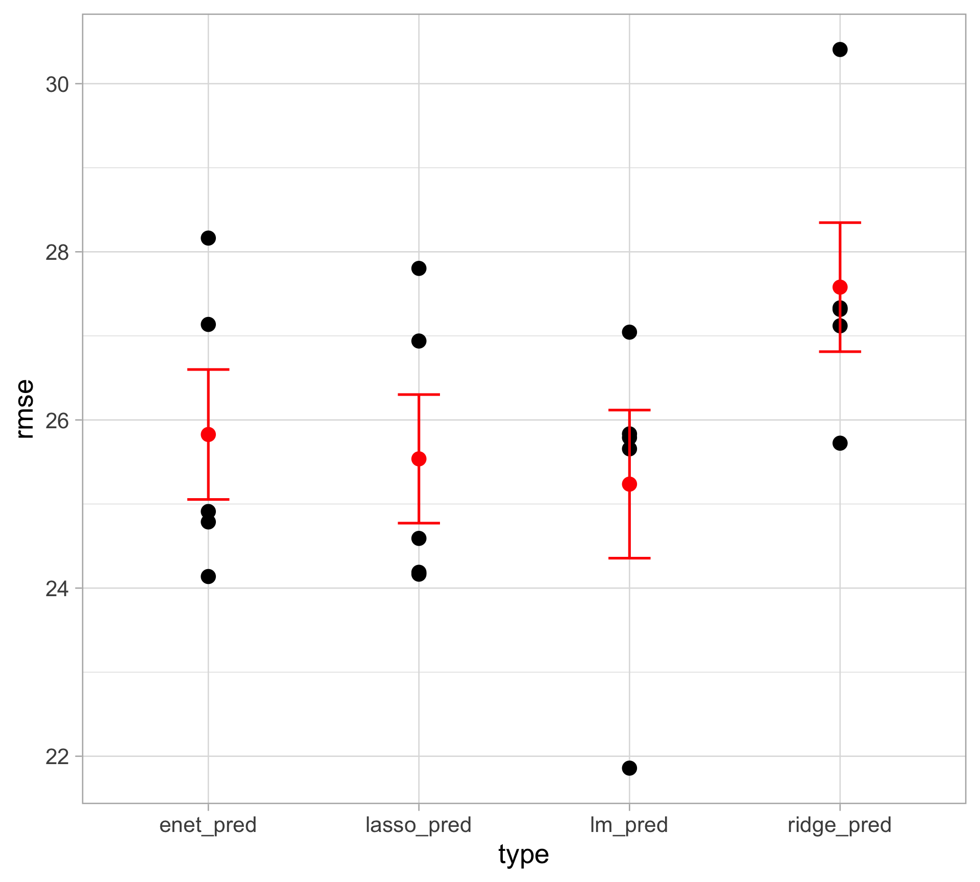
Comparison of models based on holdout performance

Compute RMSE across folds with standard error intervals

test_pred_all |>
  pivot_longer(lm_pred:enet_pred, 
               names_to = "type", 
               values_to = "test_pred") |>
  group_by(type, test_fold) |>
  summarize(
    rmse = sqrt(mean((test_actual - test_pred)^2))
  ) |> 
  ggplot(aes(x = type, y = rmse)) + 
  geom_point(size = 4) +
  stat_summary(fun = mean, geom = "point", 
               color = "red", size = 4) + 
  stat_summary(fun.data = mean_se, geom = "errorbar", 
               color = "red", width = 0.2)

Linear regression actually slightly outperforms regularization here, but within intervals

Ridge, lasso, elastic net: what to use?

• Ridge regression is particularly valuable when there are collinear predictors.

  • Ridge penalty reduces the covariance of \(\hat\beta\) by encouraging effects to be “shared” between collinear predictors, and as a result reduces the variance of predictions as well.

• LASSO is very useful when you are interested in identifying nonzero coefficients or when you may have many irrelevant features.

  • Can handle \(p >n\) case

  • For example, in statistical genetics, identifying the genes associated with a disease might be just as medically interesting as knowing the actual numerical association.

• Use elastic net when you have both highly correlated variables and a large number of potentially irrelevant features!

Appendix: Lasso and ridge in pictures

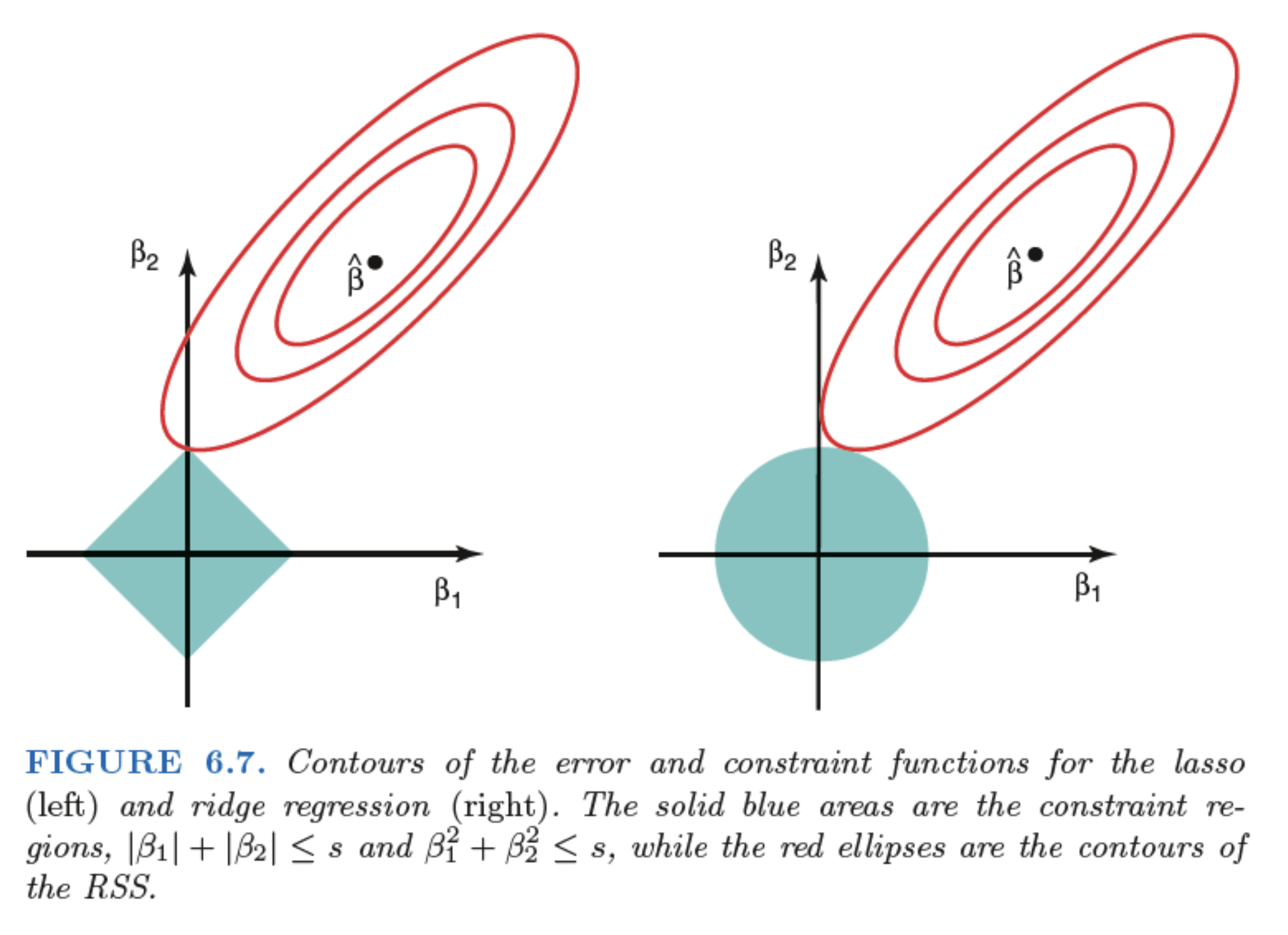
Appendix: Lasso and ridge in pictures, explained

• Consider the case of \(p=2\) (2 predictors, hence 2 coefficients \(\beta_1\) and \(\beta_2\) to be estimated)

• The residual sum of squares has elliptical contours, centered at the unregularized least squares estimate \(\hat \beta\)

• The constraint region for lasso (left) is the diamond \(\vert \beta_1 \vert + \vert \beta_2 \vert \le s\)

• The constraint region for ridge (right) is the square \(\beta_1 ^ 2 + \beta_2 ^ 2 \le s\)

• Both methods aim to find the first point where the elliptical contours hit the constraint region

• Unlike the disk, the diamond has corners; if the solution occurs at a corner, then it has one \(\beta_j\) equal to zero

• When \(p>2\), the diamond becomes a rhomboid (with many corners, flat edges, faces, etc.), allowing more opportunities for the estimated coefficients to be zero