Department of Statistics & Data Science Carnegie Mellon University
Principal Components Analysis (PCA) Recap
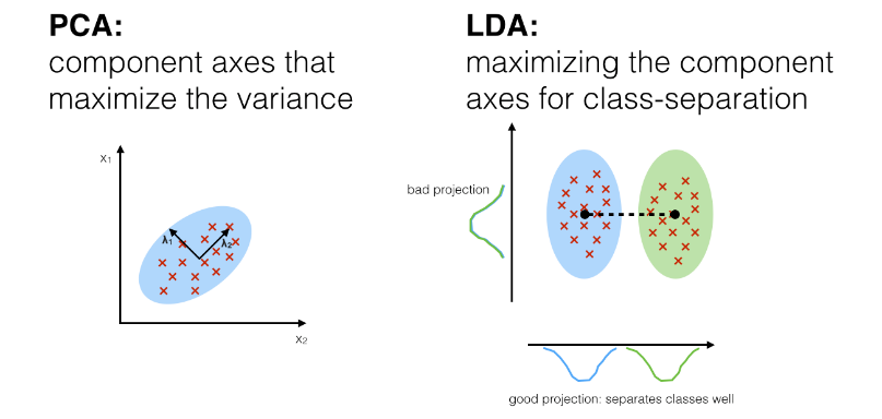
Unsupervised method of dimensionality reduction that aims to find the directions of maximum variance in a dataset
End goal is to have a smaller set of variables (principal components) that capture the most important patterns in the data. These principal components
are linear combinations of the features
are mutally uncorrelated
Keep the principal components that explain a certain percentage of the total variance in the data
Overview of LDA
Aims to find the linear combination of features that best separates the classes in a dataset
This makes LDA a supervised learning method for dimensionality reduction
End goal is to reduce the dimensionality of the data while preserving the information that is most relevant for class discrimination
Examples of problems using LDA
Based on a patient’s set of medical features, should we classify the patient as healthy or suffering from a particular disease?
Given a product’s various measurements or attributes, should we classify it as defective or non-defective?
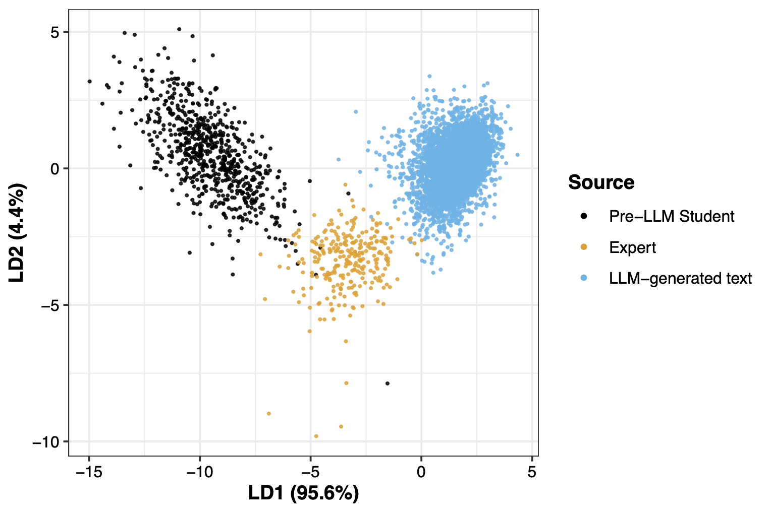
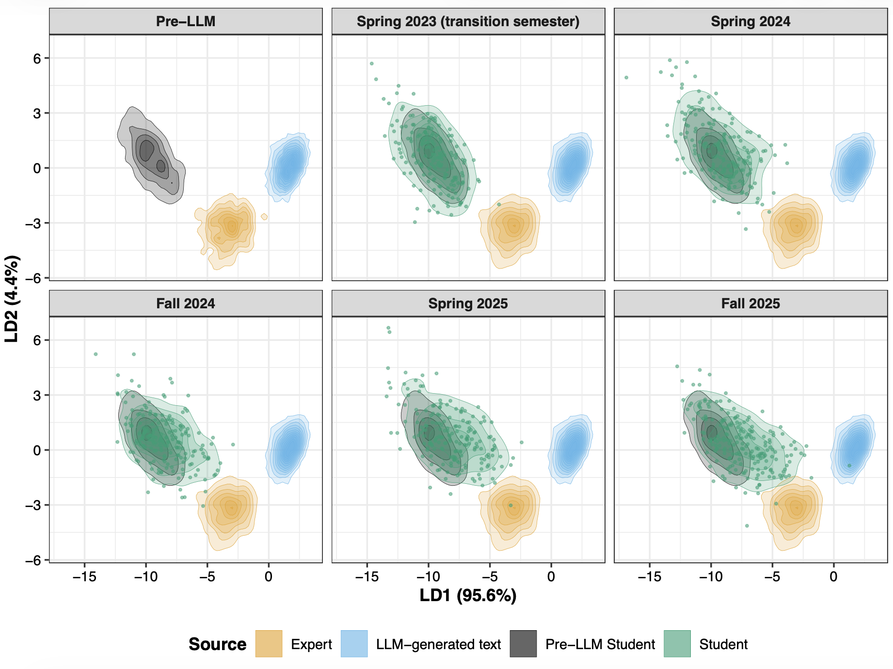
Given the a text’s set of stylistic features, is it most likely written by a student, expert, or large language model? Sara and Erin’s preprint
LDA for text classification
LDA for text classification
LDA visually
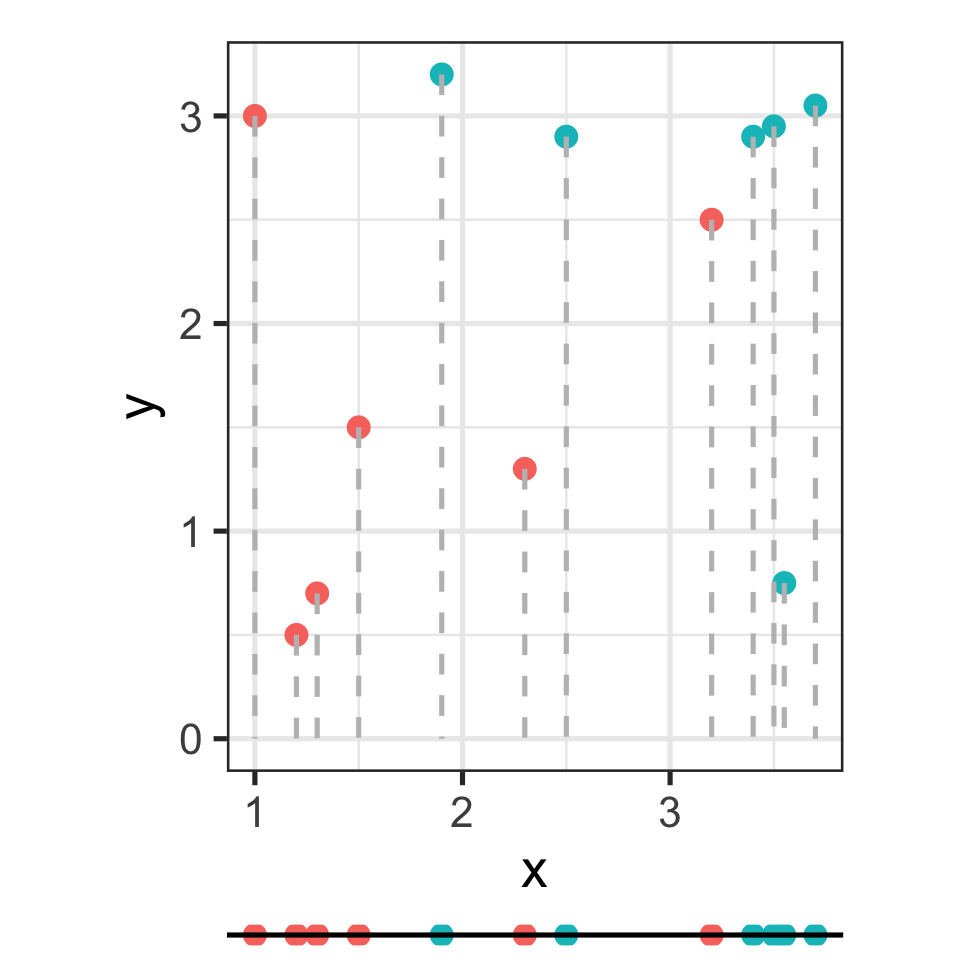
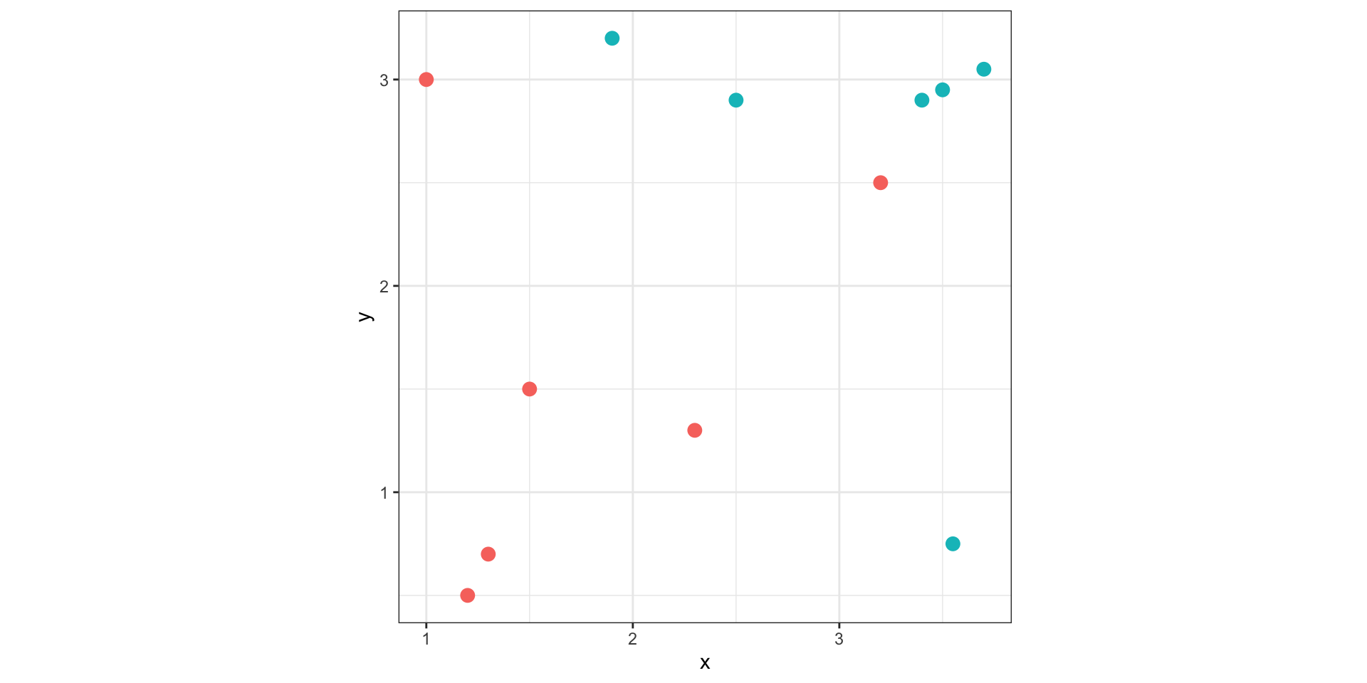
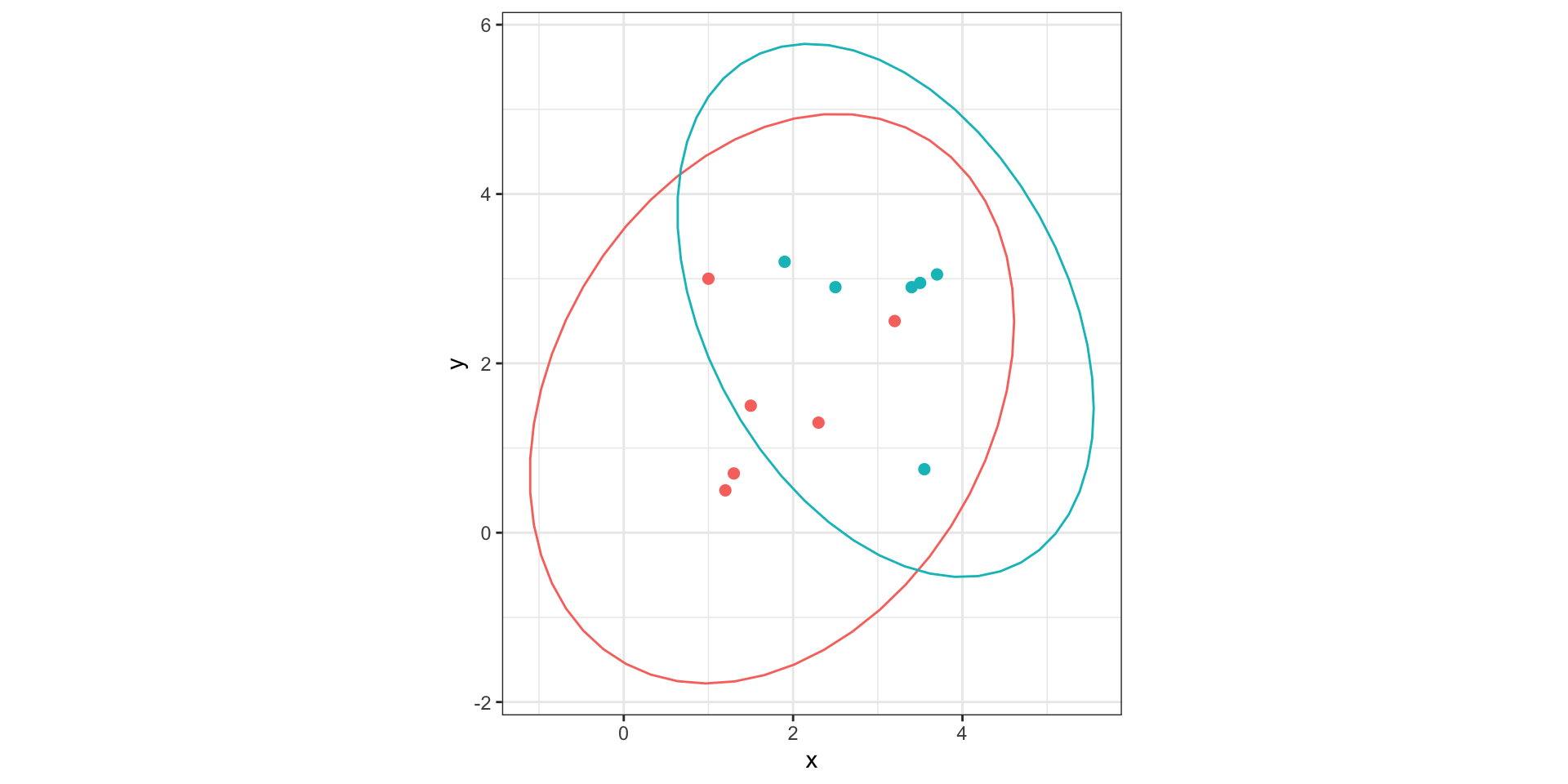
Let’s say we are interested in deciding whether to give someone a medication based on two features: \(x\) and \(y\).
Blue: responders to the medication
Red: non-responders to the medication
LDA visually
For a two-class problem, LDA finds a single projection direction that maximizes the separation between classes relative to the variation within classes.
The original data are projected onto this axis, reducing the problem from \(p\) dimensions (where \(p\) = number of predictors, here \(p=2\)) to one dimension.
What’s the best way to determine the projection direction?
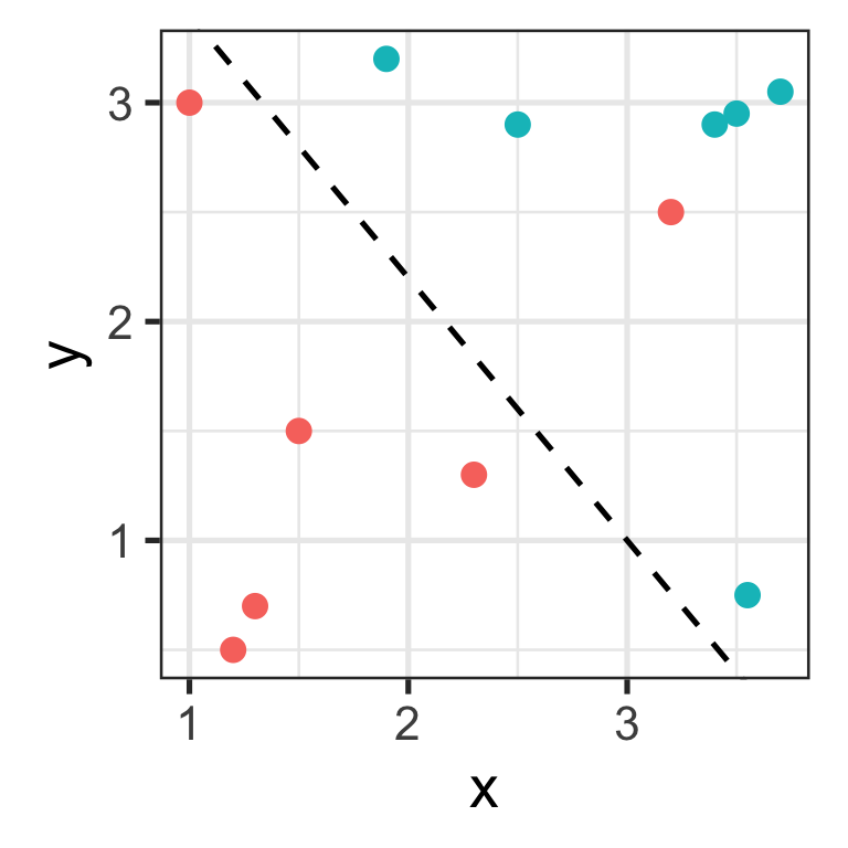
One option (bad) is to ignore \(y\) and project the data down onto the \(x\) axis.
LDA visually
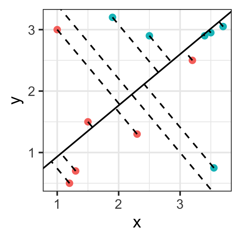
LDA finds the projection direction that produces the greatest separation between responders and non-responders
This is perpendicular to the boundary that we might draw if we were separating these points by hand (dashed line on left plot)
LDA visually
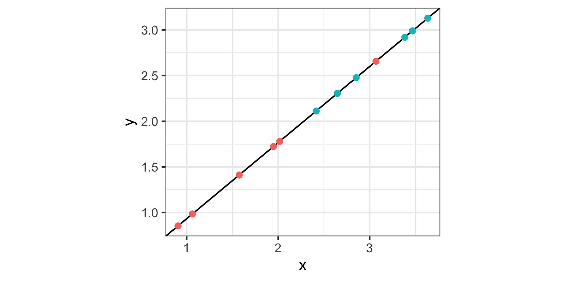
We can now see the data projected onto the new axis in a way that maximizes the separation between responders and non-responders!
Finding the “best” axis
LDA builds the model on two matrices.
First, the between-group sum-of-square matrix, which measures the differences between the class means:
The linear discriminant space is generated by computing the eigenvectors of \(W^{-1}B\).
This is the \((g-1)\)-D space where the group means are most separated with respect to the pooled variance-covariance matrix.
In other words, LDA asks which direction gives the greatest separation of the groups relative to their within-group spread.
The answer is the eigenvector corresponding to the largest eigenvalue of \(W^{-1}B\).
The pooled covariance matrix
\(W\) can be considered the pooled within-class covariance (or scatter) matrix.
LDA makes two assumptions
The cluster structure corresponding to each class forms an ellipse, showing that the class is consistent with a sample from a multivariate normal distribution
The variance of values around each mean is nearly the same. More specifically, the classes have approximately equal covariance matrices.
Let \(X\) denote the vector of predictor variables for one individual. In the toy example, \(X = (x, y)^T\)
LDA assumes that the covariance matrix \(\Sigma = \begin{pmatrix} \sigma_x^2 & \sigma_{xy} \\ \sigma_{xy} & \sigma_y^2 \end{pmatrix}\) is shared across classes.
The pooled covariance matrix
The constant covariance assumption means the multi-dimensional spread and correlation of the features are identical across groups, differing only by their central means.
LDA is known to be quite robust and often performs well even if this assumption is slightly violated.
For example, the covariance ellipses for the toy dataset are not equivalent, but we’d likely proceed with LDA.
If we have evidence the assumption is broken, we’d proceed with quadratic discriminant analysis.
Assigning observations a class
Given a new observation \(x\), for each class we compute
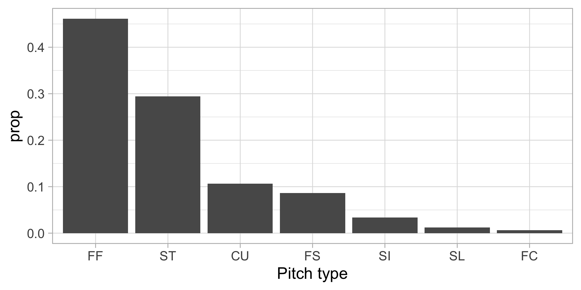
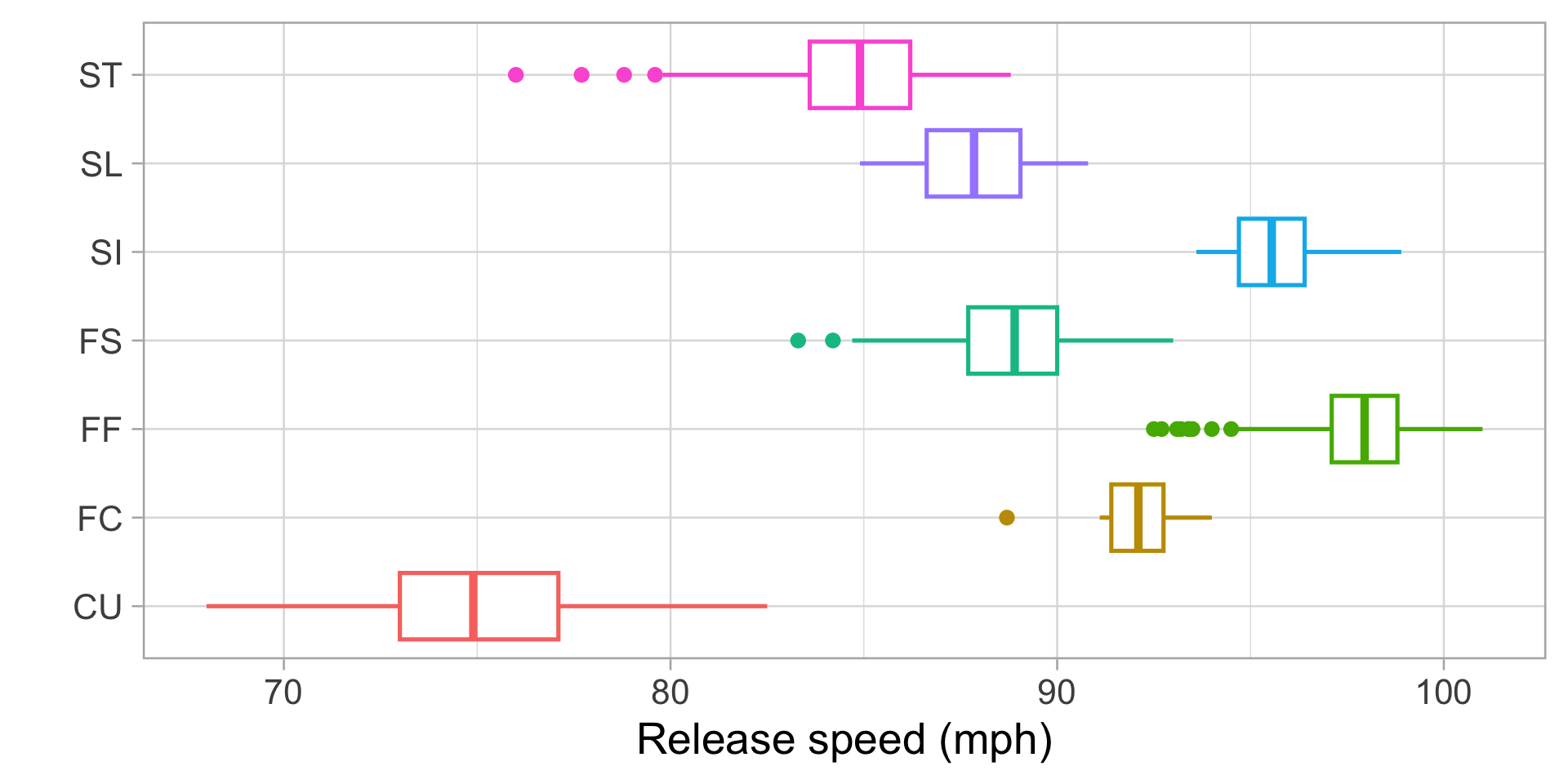
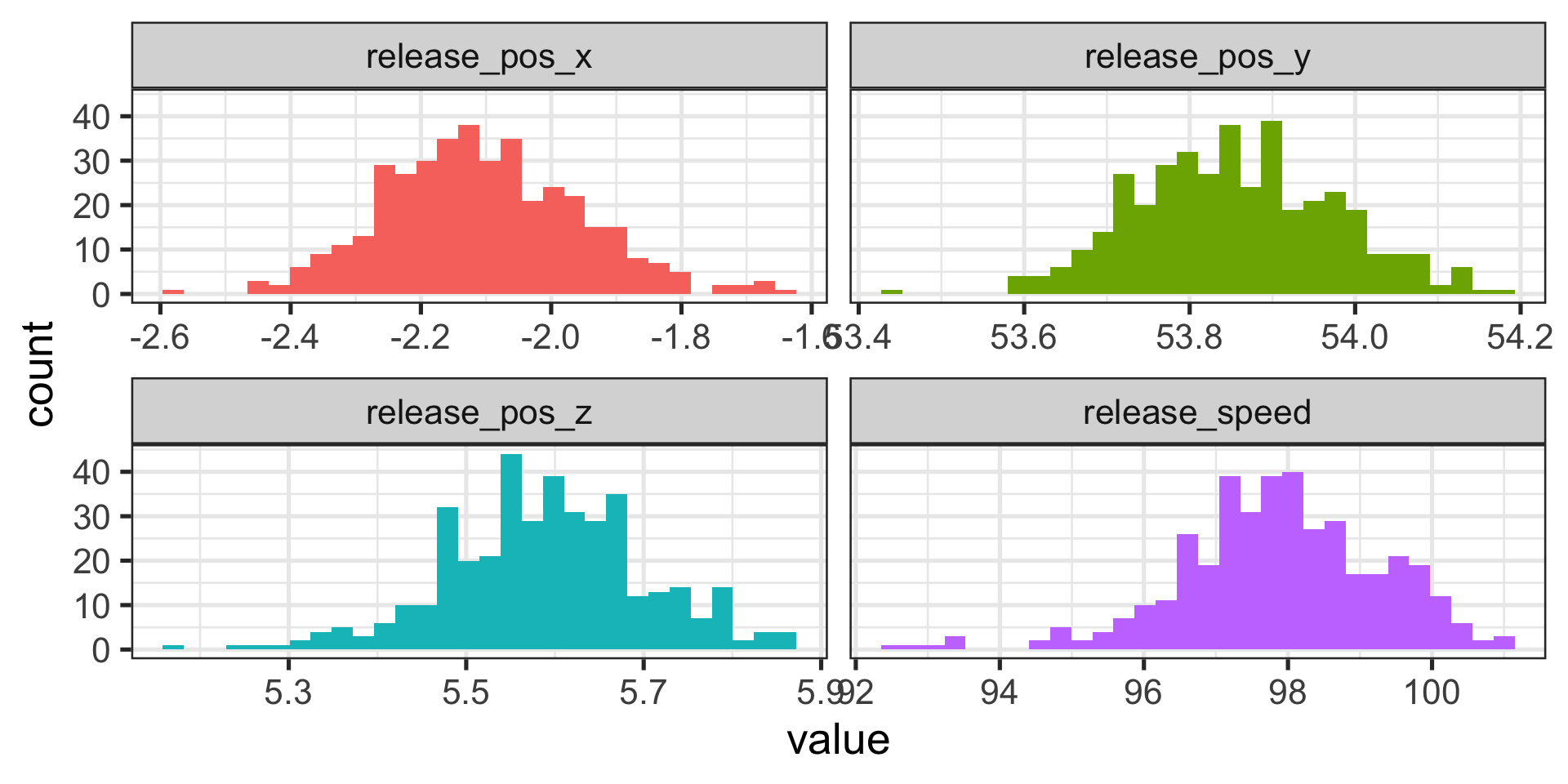
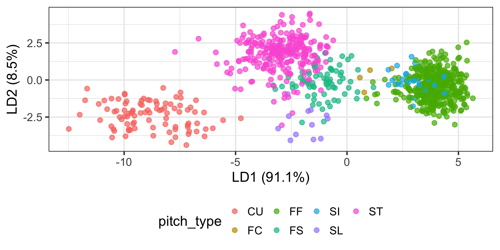
First, determine class and variables of interest. Our research question will be: can we discern Shohei Ohtani’s pitch types from his release speed and position?
To check the constant covariance assumption, we can use ellipse plots or compare covariance matrices across pitch types.
The boxM R function performs the Box’s (1949) M-test for homogeneity of covariance matrices obtained from multivariate normal data according to one or more classification factors
Keep in mind this test may reject for small differences in large sample sizes.
test_preds <-predict(lda_mod, test)$class#mean(test_preds == test$pitch_type)table(Predicted = test_preds, Actual = test$pitch_type)
         Actual
Predicted  CU  FC  FF  FS  SI  SL  ST
       CU  29   0   0   0   0   0   0
       FC   0   0   0   0   0   0   0
       FF   0   1 130   0   7   0   0
       FS   0   1   0  24   0   0   3
       SI   0   0   0   0   1   0   0
       SL   0   1   0   1   0   2   1
       ST   0   0   0   3   0   0  81
Step 5: What features contribute?
We didn’t standardize the variables beforehand, so we cannot use the size of the coefficients to understand which variables drive each axis
If we had standardized beforehand, we might be able to interpret like “A one sd increase in release speed changes the LD1 score by about X units, whereas a one sd change release height changes LD1 by only about Y units”.
However, we can calculate the correlation of the LD scores with each variable.