Supervised learning: logistic regression

CMSACamp 2026

Department of Statistics & Data Science
Carnegie Mellon University

Classification

• Categorical variables take values in an unordered set with different categories

• Classification: predicting a categorical response \(Y\) for an observation (since it involves assigning the observation to a category/class)

• Often, we are more interested in estimating the probability for each category of the response \(Y\) rather than just the class label

• Classification is different from clustering, since we know the true label \(Y\) (i.e., it is supervised learning!)

• Today, will focus on the case where we have a binary categorical response (categorical response variables with only two categories)

Logistic regression

• Recall: in linear regression, the response variable \(Y\) is quantitative/continuous

  • Examples: NFL score differential, MLB wOBA

• Logistic regression,the response variable \(Y\) is binary (i.e. \(Y \in \{0, 1\}\))

  • Examples: whether a patient has a disease, whether the kicker makes a field goal attempt

Several carry over from linear regression:

• Tests for coefficients
• Factor variables
• Interactions
• Model building procedure
• Regularization

But, other concepts are different:

• Interpretation of coefficients
• Model assumptions/diagnostics
• Model evaluation

Why not linear regression for categorical data?

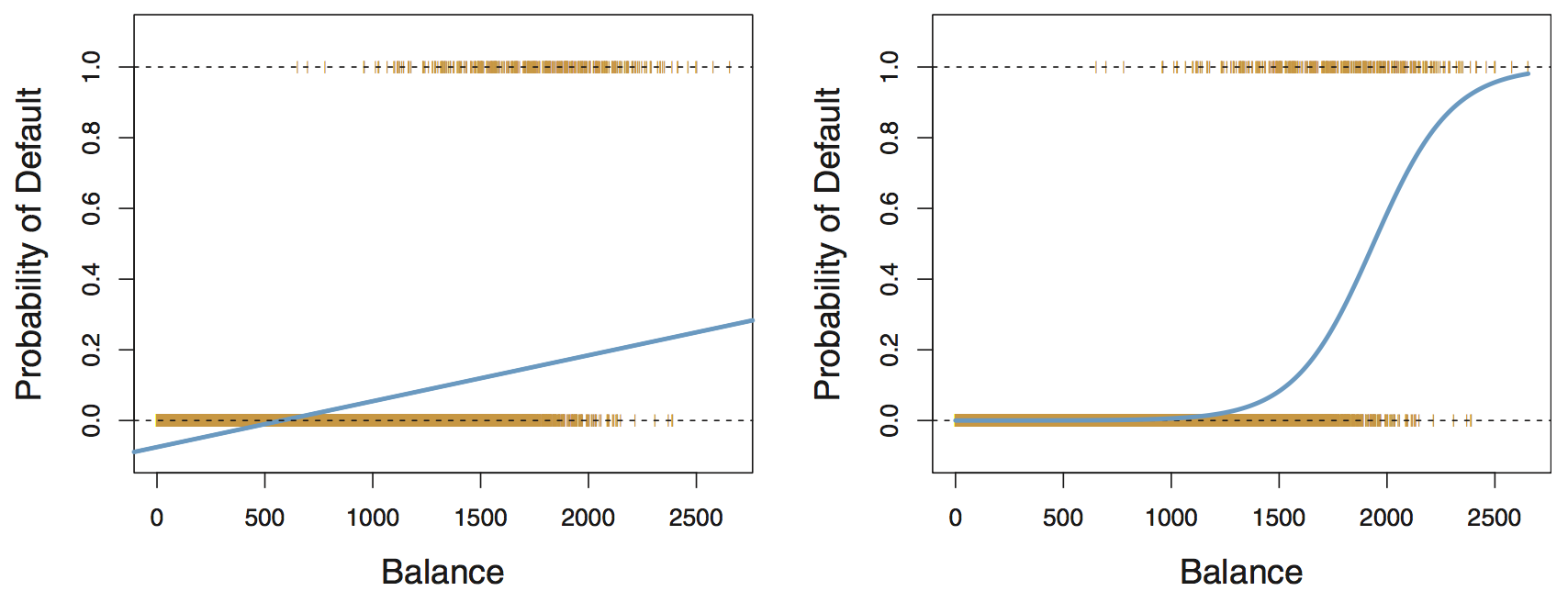
Linear regression: predicted probabilities might be outside the \([0, 1]\) interval

Logistic regression: ensures all probabilities lie between 0 and 1

Logistic regression

• Logistic regression models the probability of success \(p(x)\) of a binary categorical response variable \(Y \in \{0, 1\}\)

• To limit the regression between \([0, 1]\), we use the logit function, or the log-odds ratio

\[ \log \left( \frac{p(x)}{1 - p(x)} \right) = \beta_0 + \beta_1 x_1 + \cdots + \beta_p x_p \]

or equivalently,

\[ p(x) = \frac{e^{\beta_0 + \beta_1 x_1 + \cdots + \beta_p x_p}}{1 + e^{\beta_0 + \beta_1 x_1 + \cdots + \beta_p x_p}} \]

Note: \(p(x)= P(Y = 1 \mid X = x) = \mathbb E[Y \mid X = x]\) (aka the expected value of the outcome given the regressors!)

Model assumptions

From the last slide, we have that:

\[ \log \left( \frac{E[Y \mid X = x]}{1 - E[Y \mid X = x]} \right) = \beta_0 + \beta_1 x_1 + \cdots + \beta_p x_p \]

This encodes two model assumptions:

1. The log-odds (on the LHS) is linearly related to the regressors (on the RHS)

2. The observations \(Y_i\) are conditionally independent given the covariates \(X_i\) (like with linear regression, the best way to evaluate this assumption is with domain knowledge)

And again, we assume \(X\) is fixed, not random

Maximum likelihood estimation (MLE)

Likelihood function: how likely to observe data for given parameter values \[L(\theta) = \prod_{i=1}^n f(y_i; \theta)\]

Goal: find values for parameters that maximize likelihood function (i.e., MLEs)

• Why: likelihood methods can handle variety of data types and assumptions

• How: typically numerical approaches and optimization techniques

  • Easier to work with log-likelihood (sums compared to products)

Example: linear regression MLE

Probability density function (pdf) for a normal distribution

\[ f(y \mid \mu, \sigma) = \frac{1}{\sqrt{2\pi \sigma^2}} e^{\frac{-(y - \mu) ^ 2}{2 \sigma^2}} \]

Consider a simple linear regression model (with an intercept and one predictor) \[y_i = \beta_0 + \beta_1 x_i + \epsilon_i, \quad \epsilon_i \sim N(0, \sigma^2)\]

Then: \(\qquad \displaystyle L(\beta_0, \beta_1, \sigma) = \prod_{i=1}^n f(y_i \mid x_i; \beta_0, \beta_1, \sigma) = \prod_{i=1}^n \frac{1}{\sqrt{2\pi \sigma^2}} e^{\frac{-(y_i - \beta_0 - \beta_1 x_i) ^ 2}{2 \sigma^2}}\)

and \(\qquad \displaystyle \log L(\beta_0, \beta_1, \sigma) = -\frac{n}{2} \log 2\pi - \frac{n}{2} \log \sigma^2 - \frac{1}{2 \sigma^2} \sum_{i=1}^n (y_i - \beta_0 - \beta_1x_1)^2\)

We can then use optimization methods (e.g., calculus) to find the optimal parameter values.

For more details, see Cosma Shalizi’s notes on MLE for SLR

Logistic regression estimation

Logistic regression involves numerical optimization

• \(y_i\) is observed response for \(n\) observations, either 0 or 1

• We need to use an iterative algorithm to find \(\beta\)’s that maximize the likelihood

\[ \prod_{i=1}^{n} p\left(x_{i}\right)^{y_{i}}\left(1-p\left(x_{i}\right)\right)^{1-y_{i}} \]

• Newton’s method: start with initial guess, calculate gradient of log-likelihood, add amount proportional to the gradient to parameters, moving up log-likelihood surface

Inference with logistic regression

• Major motivation for logistic regression (and all GLMs) is inference

  • How does the response change when we change a predictor by one unit?

• For linear regression, the answer is straightforward

\[E[Y \mid X = x] = \beta_0 + \beta_1 x_1 + + \cdots + \beta_p x_p\]

• For logistic regression, it is a little less straightforward

\[E[Y \mid X = x] = \frac{e^{\beta_0 + \beta_1 x_1 + \cdots + \beta_p x_p}}{1 + e^{\beta_0 + \beta_1 x_1 + \cdots + \beta_p x_p}}\]

Note: (i) the predicted response varies non-linearly with the predictor variable values, and (ii) interpretation on the odds scale

The odds interpretation

The odds of an event is the probability of the event occurring divided by the probability of the event not occurring

\[ \displaystyle \text{odds} = \frac{\text{probability}}{1 - \text{probability}} = \frac{p(x)}{1 - p(x)} \]

We can solve to obtain to probability:

\[ p(x) = \displaystyle \text{probability} = \frac{\text{odds}}{1 + \text{odds}} \]

Example: Rolling a fair six-sided die

• The probability of rolling a 2 is 1/6

• The odds of rolling a 2 is 1/5 (aka 1-to-5 or 1:5)

The odds interpretation

Suppose we fit a simple logistic regression model (with one predictor), and say the predicted probability is 0.8 for a particular predictor value (\(X = x\))

• This means that if we were to repeatedly sample response values given that predictor variable value: we expect class 1 to appear 4 times as often as class 0 \[\text{odds} = \frac{E[Y \mid X = x] }{1-E[Y \mid X = x] } = \frac{0.8}{1-0.8} = 4 = e^{\beta_0+\beta_1x}\]

• Thus we say that for the given predictor variable value, the odds are 4 (or 4:1) in favor of class 1

How does the odds change if we change the value of a predictor variable by one unit?

\[\text{odds}_{\rm new} = e^{\beta_0+\beta_1(x+1)} = e^{\beta_0+\beta_1x}e^{\beta_1} = e^{\beta_1}\text{odds}_{\rm old}\]

For every one-unit increase in \(x\), the odds change by a factor of \(e^{\beta_1}\)

Example in R

Background on cricket

For some background on cricket, see this overview. Particularly relevant for us:

• Each time the two batters switch sides without getting out counts as a single run scored

• If the batter hits the ball on a bounce to the oval boundary, it counts as four runs scored

• If the batter hits the ball over the oval boundary on a fly, it counts as six runs scored

• An extra run is a run that is awarded to the batting team that is not credited to any individual batter (e.g., illegal deliveries, no-ball, wide)

See: highlights from the Final - India vs Pakistan in Asia Cup 2025

Data: Asia Cup Cricket Results

Each observation represents a cricket match played in the Asia Cup between 1984–2022

• team: focal team (opponent: non-focal team)

• result: whether or not the focal team won/lost the match

• selection: focal team’s selection (batting or bowling) after winning/losing the toss

• fours: total scored fours for that team

• sixes: total scored sixes for that team

• extras_scored: number of extra runs given up

• given_extras: number of extra runs scored

library(tidyverse)
theme_set(theme_light())

cricket <- read_csv("https://raw.githubusercontent.com/36-SURE/2026/main/data/cricket_asia_cup.csv") |>
  janitor::clean_names() |>
  mutate(selection = as_factor(if_else(selection == 1, "Bowling" , "Batting")),
         result = as_factor(if_else(result == 1, "Win", "Loss")))

Fitting a logistic regression model

Use the glm function, specifying the family as binomial

Get coefficients table using the tidy() function in the broom package (on log-odds scale)!

cricket_logit <- glm(result ~ selection + fours + sixes +
                       extras_scored + given_extras, data = cricket, family = binomial)

library(broom)
tidy(cricket_logit)

# A tibble: 6 × 5
  term             estimate std.error statistic   p.value
  <chr>               <dbl>     <dbl>     <dbl>     <dbl>
1 (Intercept)       -1.92      0.489      -3.92 0.0000894
2 selectionBowling   0.494     0.276       1.79 0.0730   
3 fours              0.0804    0.0209      3.84 0.000122 
4 sixes              0.128     0.0605      2.12 0.0343   
5 extras_scored     -0.0213    0.0193     -1.10 0.270    
6 given_extras       0.0222    0.0197      1.13 0.259    

Interpreting a logistic regression model

library(gtsummary)
# tidy(cricket_logit, conf.int = TRUE, exponentiate = TRUE)
tbl_regression(cricket_logit, exponentiate = TRUE)

Characteristic	OR	95% CI	p-value
selection
Batting	—	—
Bowling	1.64	0.96, 2.83	0.073
fours	1.08	1.04, 1.13	<0.001
sixes	1.14	1.01, 1.28	0.034
extras_scored	0.98	0.94, 1.02	0.3
given_extras	1.02	0.98, 1.06	0.3
Abbreviations: CI = Confidence Interval, OR = Odds Ratio

Examples interpretations

selection: the odds ratio is 1.64

In the Asia Cup, bowling instead of batting first is associated with an increase in the odds of winning the match by a multiplicative factor of 1.64 (95% CI [0.96, 2.83]).

fours: the odds ratio is 1.08

In the Asia cup, each additional scored four is associated with an increase in the odds of winning the match by a multiplicative factor of 1.08 (95% CI [1.04, 1.13]).

Linearity EDA: empirical link plot

Recall: logistic regression assumes that the log-odds is linearly related to the regressors

library(regressinator)

rate_by_fours <- cricket |>
  mutate(win = (result == "Win")) |>
  bin_by_quantile(fours, breaks = 10) |>
  summarize(
    mean_fours = mean(fours),
    prob = mean(win),
    log_odds = empirical_link(
      win,
      family = binomial(link = "logit")),
    n = n()
  )

rate_by_fours |>
  ggplot(aes(x = mean_fours, y = log_odds)) +
  geom_point(aes(size = n)) +
  geom_smooth() +
  labs(x = "Number of fours scored", y = "log-odds of winning")

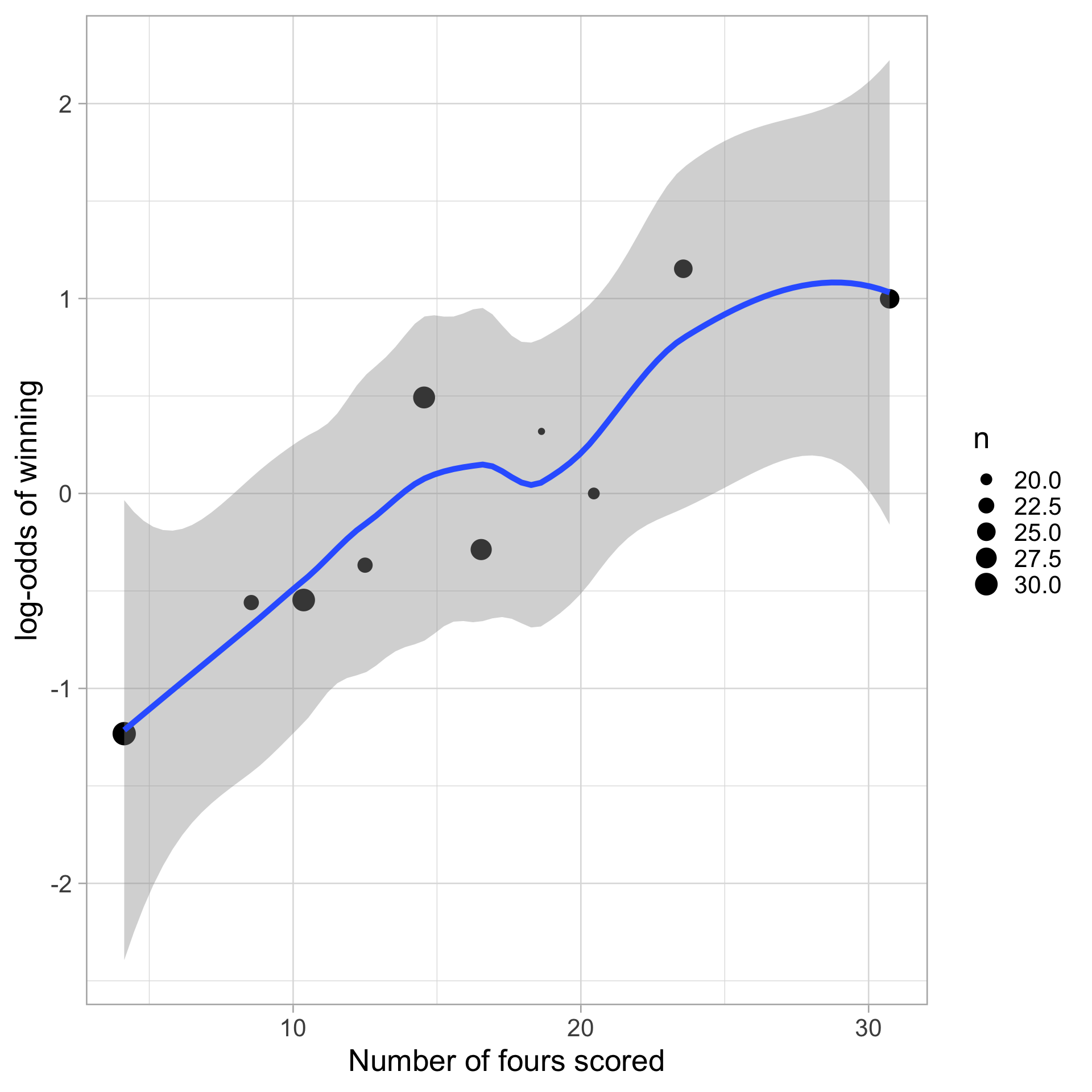
Diagnosing (non-)linearity

Similar to linear regression: can use a fitted versus residual plot to diagnose (non)-linearity

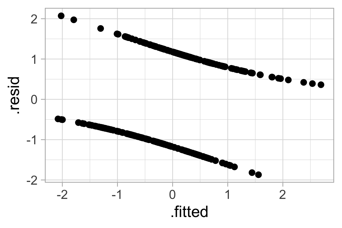
BUT, unlike linear regression: raw residuals will look weird since \(Y_i \in \{0, 1\}\)

augment(cricket_logit) |>
  ggplot(aes(x = .fitted, y = .resid)) +
  geom_point() 

Diagnosing (non-)linearity

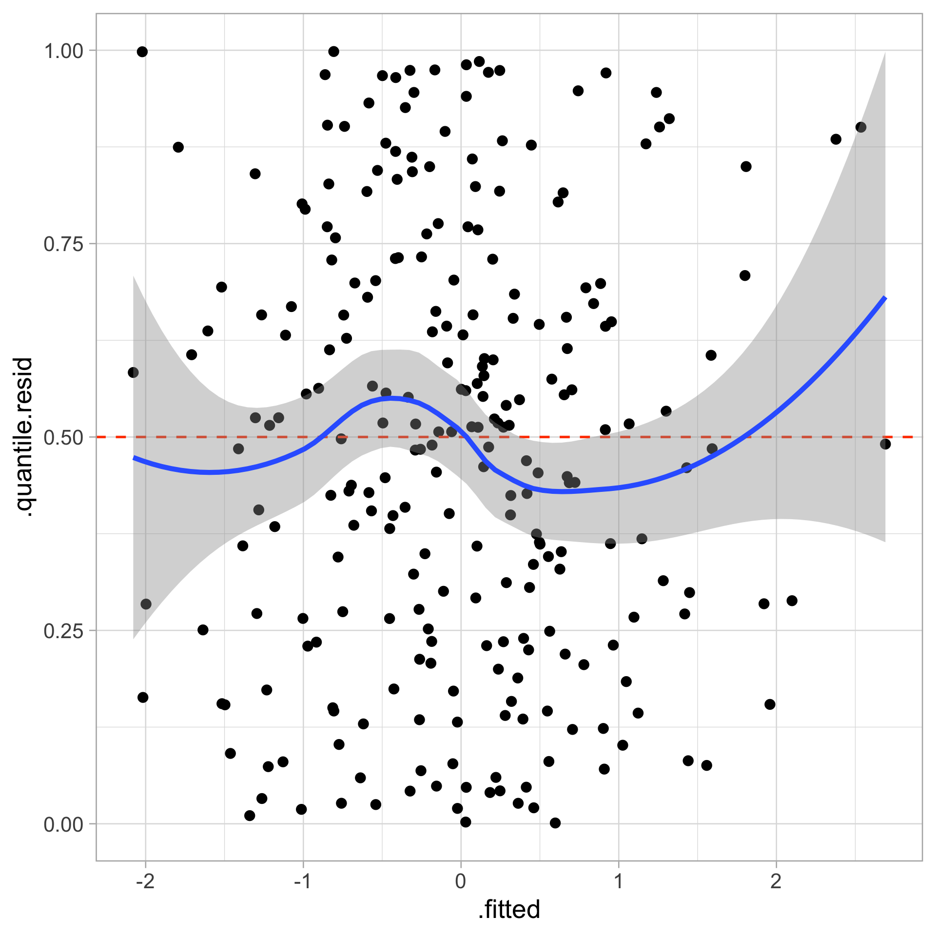
We can use randomized quantile residuals

library(DHARMa) #install.packages("DHARMa")
dh <- simulateResiduals(cricket_logit)

cricket_aug <- augment(cricket_logit) |>
  mutate(.quantile.resid = residuals(dh))

cricket_aug |>
  ggplot(aes(x = .fitted, y = .quantile.resid)) +
  geom_point() +
  geom_hline(yintercept = 0.5, color = "orangered",
             linetype = "dashed") +
  geom_smooth()

• If the model is correctly specified: for each fitted value, the mean of the randomized quantile residuals will be 0.5

• Deviations from this indicate there is non-linearity between the log-odds and the regressors

Prediction

• The default output of predict() is on the log-odds scale

• To get predicted probabilities, we need to specify type = "response"

cricket_pred_prob <- predict(cricket_logit, type = "response")

But, how do we predict the class (i.e., win vs. loss)?

• Typically if the predicted probability is > 0.5 then we predict Win, else Loss (could also be encoded as 1 and 0)

cricket_pred_class <- ifelse(cricket_pred_prob > 0.5, "Win", "Loss")
cricket_pred_binary <- ifelse(cricket_pred_prob > 0.5, 1, 0)

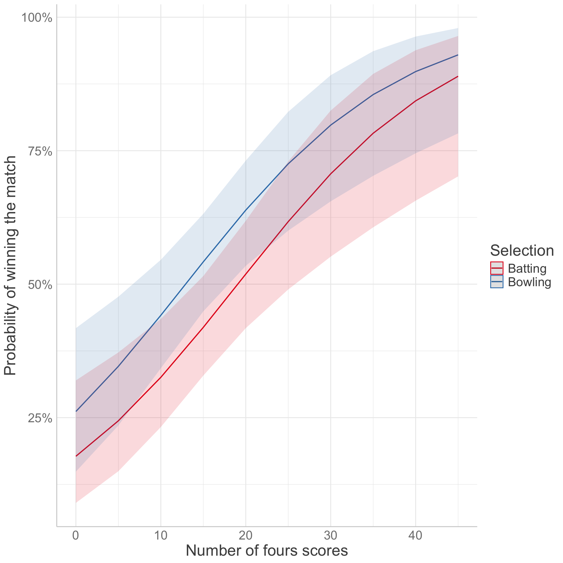
Effect plots for the predicted probability

library(ggeffects) #install.packages("ggeffects")

predict_response(cricket_logit,
                 terms = c("fours", "selection")) |>
  plot() +
  labs(x = "Number of fours scores",
       y = "Probability of winning the match",
       color = "Selection", title = NULL) 

Deviance

• In linear regression, we have the residual sum of squares (RSS)—an RSS of zero means the model predicts perfectly

• In logistic regression, the RSS is less meaningful since our outcome is binary, not a probability

• Instead we define the deviance as a measure of goodness-of-fit

  • Generalization of RSS in linear regression to any distribution family

For more details, see Wikipedia page on Deviance in Statistics

Deviance

For model of interest \(\mathcal{M}\) the total deviance is:

\[D_{\mathcal{M}}= -2 \log \frac{\mathcal{L}_{\mathcal{M}}}{\mathcal{L}_{\mathcal{S}}} = 2\left(\log \mathcal{L}_{\mathcal{S}}-\log \mathcal{L}_{\mathcal{M}}\right)\]

where:

• \(\mathcal{L}_{\mathcal{M}}\) is the likelihood for model \(\mathcal{M}\)

• \(\mathcal{L}_{\mathcal{S}}\) is the likelihood for the saturated model (i.e., the most complex model possible, providing a perfect fit to the data)

Deviance is a measure of goodness-of-fit: the smaller the deviance, the better the model fit

glance(cricket_logit)

# A tibble: 1 × 8
  null.deviance df.null logLik   AIC   BIC deviance df.residual  nobs
          <dbl>   <int>  <dbl> <dbl> <dbl>    <dbl>       <int> <int>
1          349.     251  -156.  325.  346.     313.         246   252

Classification model assessment

Misclassification rate

mean(cricket_pred_class != cricket$result)

[1] 0.3293651

prop.table(table(cricket$result)) # should always check the class balance!

     Loss       Win 
0.5079365 0.4920635 

Brier score (similar to MSE for regression – the lower, the better calibrated predictions)

mean((cricket_pred_binary - cricket_pred_prob)^2)

[1] 0.132667

Confusion matrix

table("Predicted" = factor(cricket_pred_class, levels = c("Win", "Loss")), 
      "Observed" = factor(cricket$result, levels = c("Win", "Loss")))

         Observed
Predicted Win Loss
     Win   83   42
     Loss  41   86

Ideally, all of these should be calculated on held-out predictions (not just the training sample!)

Confusion matrix

Actual Class	Predicted class
	P (1)	N (0)
P (1)	True Positives (TP)	False Negatives (FN)
N (0)	False Positives (FP)	True Negatives (TN)

• Accuracy: How often is the classifier correct? \((\text{TP} + \text{TN}) \ / \ {\text{total}}\)

• Precision: How often is it right for predicted positives? \(\text{TP} \ / \ (\text{TP} + \text{FP})\)

• Sensitivity (aka true positive rate (TPR) or power): How often does it detect positives? \(\text{TP} \ / \ (\text{TP} + \text{FN})\)

• Specificity (aka true negative rate (TNR), or 1 - false positive rate (FPR)): How often does it detect negatives? \(\text{TN} \ / \ (\text{TN} + \text{FP})\)

There are a ton of other metrics…

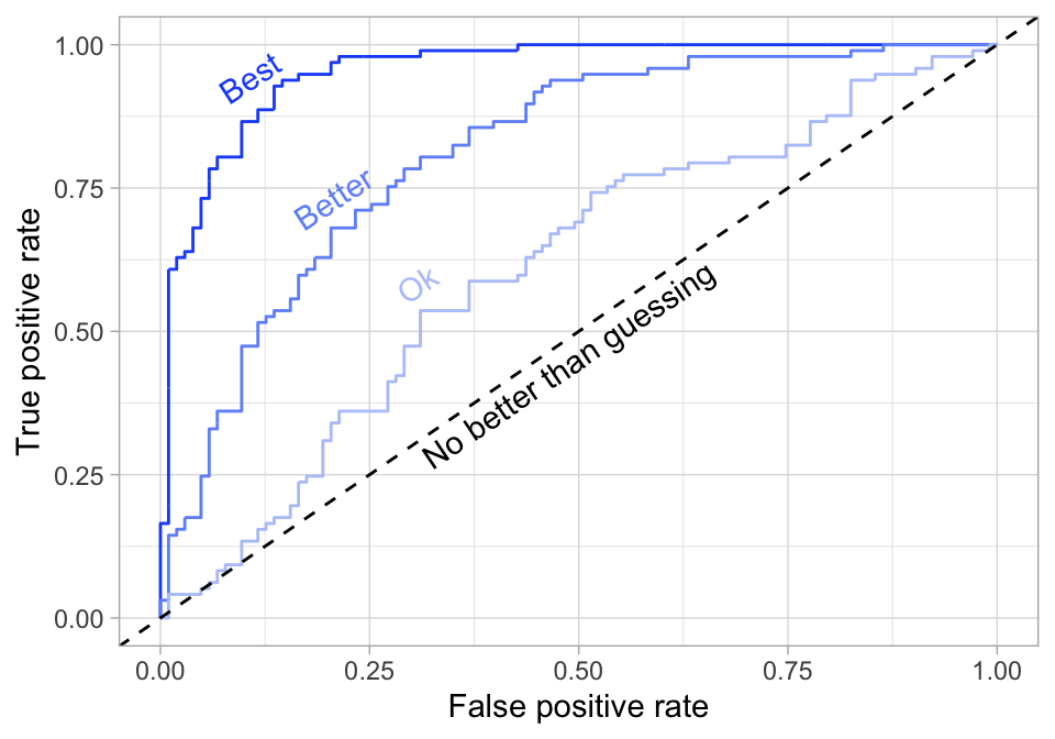
Receiver operating characteristic (ROC) curve

Question: How do we balance between high power and low false positive rate?

• In general, we can obtain predicted class for each observation by comparing the predicted probability to some cutoff \(c\) (typically, \(c=0.5\)) \[\hat{Y} =\left\{\begin{array}{ll} 1, & \hat{p}(x)>c \\ 0, & \hat{p}(x) \leq c \end{array}\right.\]

• ROC curve: check all possible values for the cutoff \(c\), plot the power against false positive rate

We use the optimal \(c\) as the class cut-off for held-out/unseen test data (basically, treat the cut-off \(c\) as a tuning parameter)

Receiver operating characteristic (ROC) curve

We want to maximize the area under the curve (AUC)

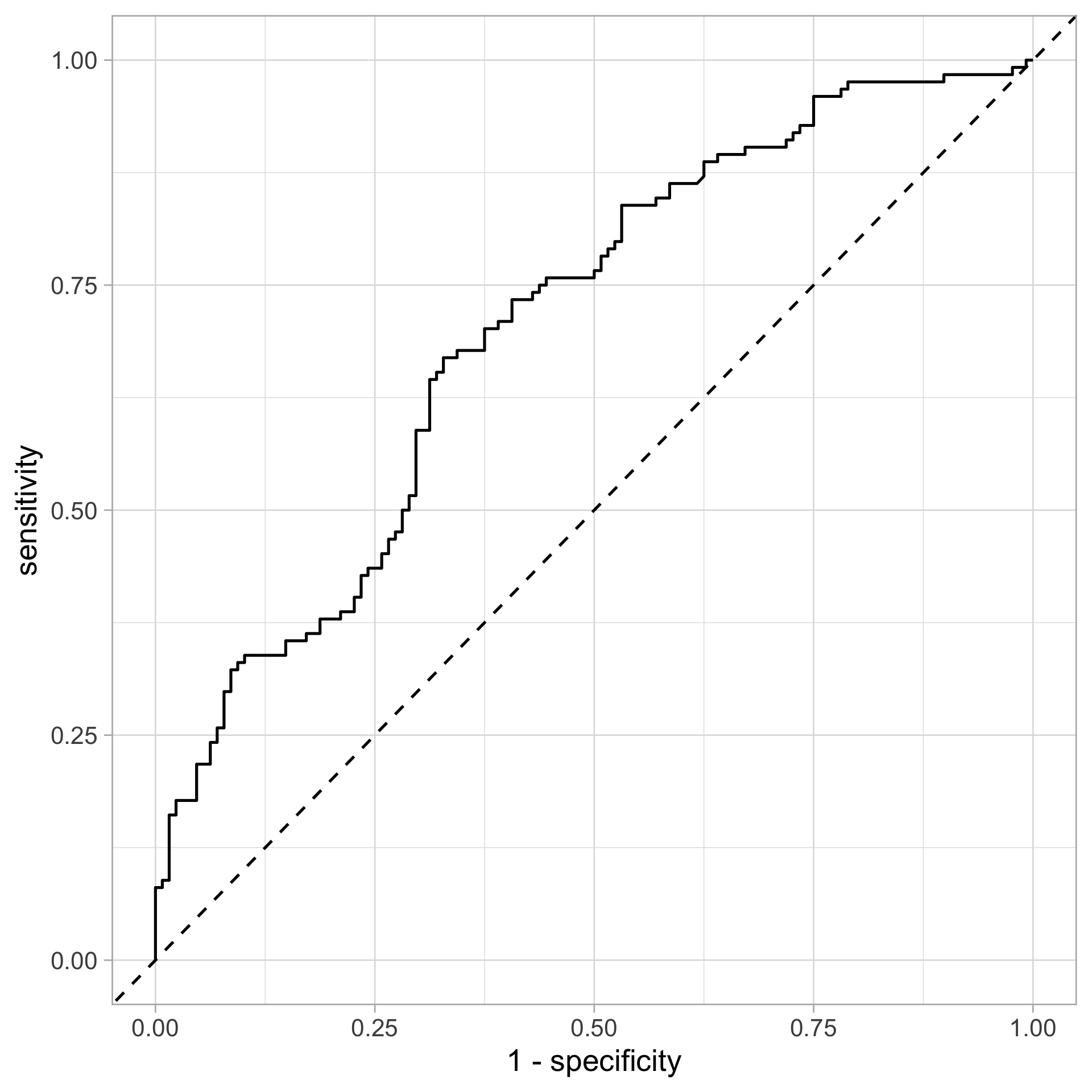
Calculating AUC & plotting an ROC curve

library(pROC)
cricket_roc <- cricket |> 
  mutate(pred_prob = predict(cricket_logit, 
                             type = "response")) |> 
  roc(result, pred_prob)
# str(cricket_roc)
cricket_roc$auc

Area under the curve: 0.7034

tibble(threshold = cricket_roc$thresholds,
       specificity = cricket_roc$specificities,
       sensitivity = cricket_roc$sensitivities) |> 
  ggplot(aes(x = 1 - specificity, y = sensitivity)) +
  geom_path() +
  geom_abline(slope = 1, intercept = 0, 
              linetype = "dashed")

Calibration

• Classification models go beyond providing binary predictions and instead produce predicted probabilities for each class

• It might be desirable to assess the quality of the predicted probabilities instead of just the accuracy of the crude predicted class labels

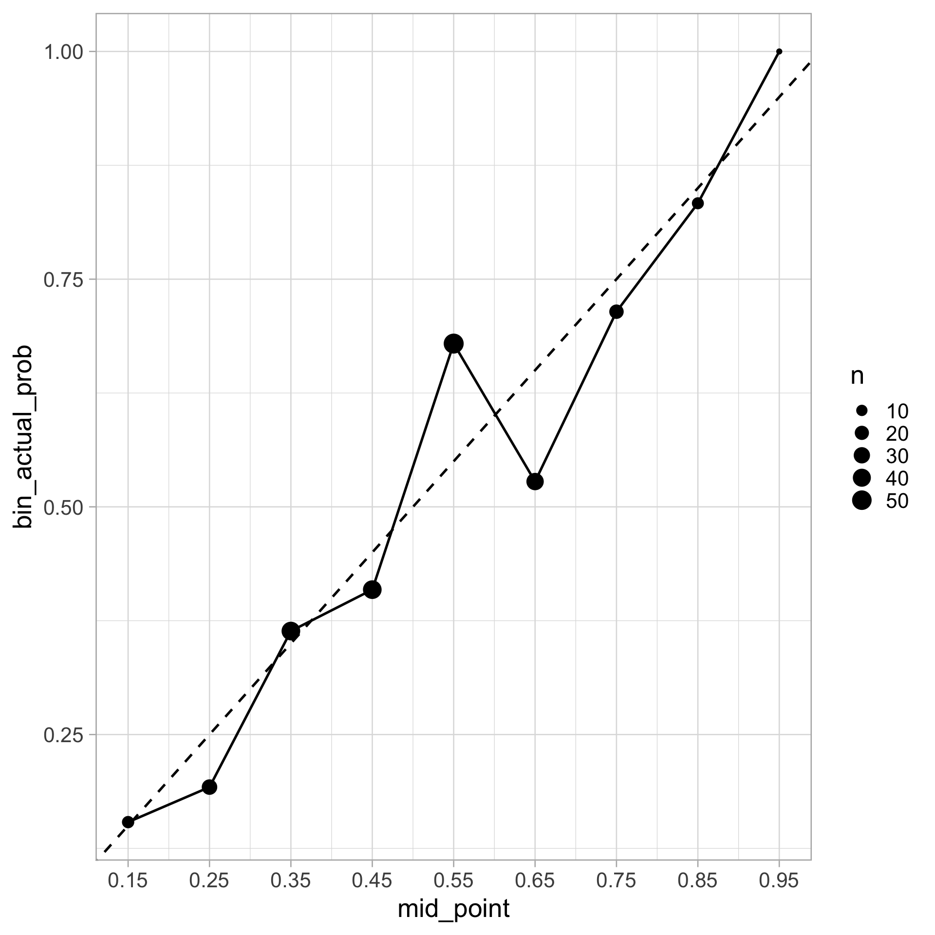
• A model is well-calibrated if the predicted probabilities match the actual probabilities (actual likelihood of an event occurring)

  • Example of an uncalibrated model: if we’ve got a model which tells us that the probability of rain on a certain class of days is 50%, it better rain on half of those days in reality, or the model is wrong about the probability of rain

Note: calibration should be used together with other model evaluation and diagnostic tools

• A model can well-calibrated but bad at making predictions (example: a classifier that always predicts the base rate)

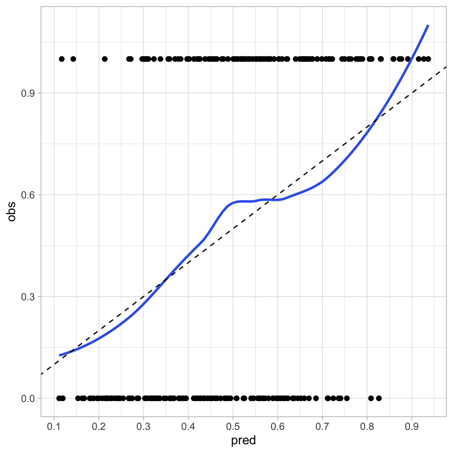
Calibration plot: smoothing

Plot the observed outcome against the fitted probability, and apply a smoother

cricket |> 
  mutate(pred = predict(cricket_logit, type = "response"),
         obs = ifelse(result == "Win", 1, 0)) |> 
  ggplot(aes(pred, obs)) +
  geom_point() +
  geom_smooth(se = FALSE) +
  geom_abline(slope = 1, intercept = 0,
              linetype = "dashed") +
  scale_x_continuous(breaks = seq(0, 1, by = 0.1))

Looks good for the most part:

• Weird behavior for high probability values

• Since there are only a few observations with high predicted probability (\(>0.85\))

Calibration plot: binning

cricket |> 
  mutate(
    pred_prob = predict(cricket_logit, type = "response"),
    bin_pred_prob = cut(pred_prob, breaks = seq(0, 1, .1))
  ) |> 
  group_by(bin_pred_prob) |> 
  summarize(n = n(),
            bin_actual_prob = mean(result == "Win")) |> 
  mutate(mid_point = seq(0.15, 0.95, 0.1)) |> 
  ggplot(aes(x = mid_point, y = bin_actual_prob)) +
  geom_point(aes(size = n)) +
  geom_line() +
  geom_abline(slope = 1, intercept = 0, 
              color = "black", linetype = "dashed") +
  scale_x_continuous(breaks = seq(0.15, 0.95, 0.1)) 
  # expand_limits(x = c(0, 1), y = c(0, 1))

Other calibration methods

• Platt scaling

• Isotonic regression

• Beta calibration

• probably package in R

• Formally, a classifier is calibrated (or well-calibrated) when \(P(Y = 1 \mid\hat p(X) = p) = p\)

Comparing methods

What do you think are the pros or cons of logistic regression compared to LDA? When might you use each method?