Supervised learning: nonparametric regression

CMSACamp 2026

Department of Statistics & Data Science
Carnegie Mellon University

Background

Recall: Model flexibility vs interpretability

Generally speaking: trade-off between a model’s flexibility (i.e. how “wiggly” it is) and how interpretable it is

Parametric methods (e.g. linear regression, GLMs): we make an assumption about the functional form, or shape, of \(f\) before observing the data

Nonparametric methods: we do not make explicit assumptions about the functional form of \(f\) (i.e., \(f\) is estimated from the data)

Parametric models are generally easier to interpret, whereas nonparametric models are more flexible

\(k\)-nearest neighbors (\(k\)-NN)

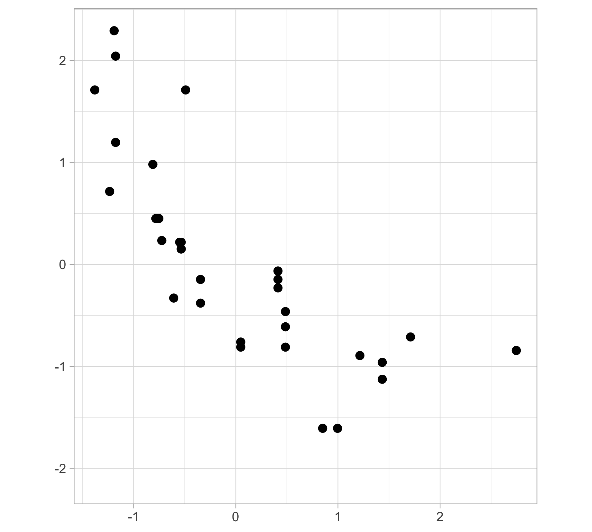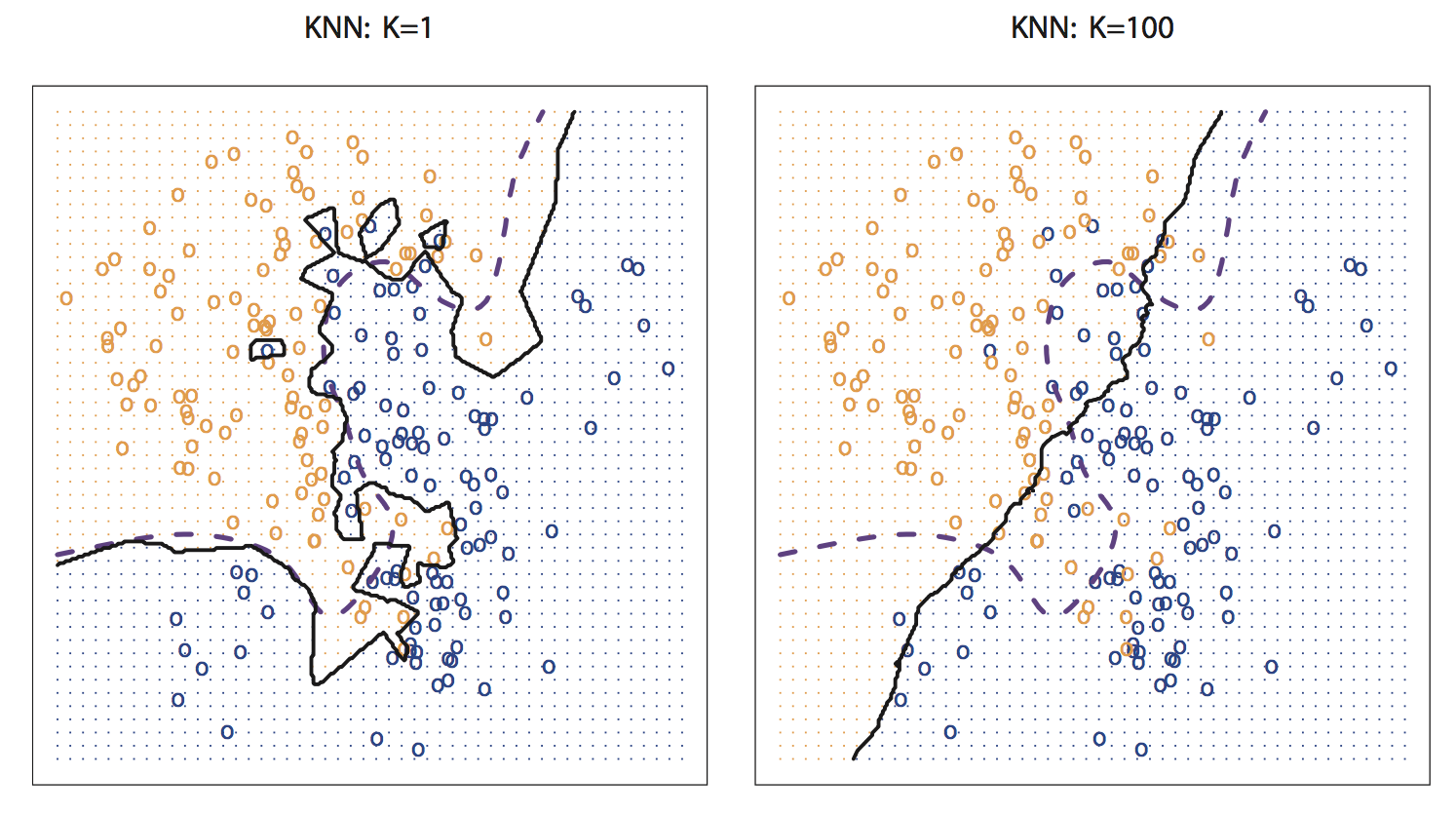
Find the \(k\) data points closest to an observation \(x\), use these to make predictions
- Need to use some measure of distance, e.g., Euclidean distance

Take the average value of the response over the \(k\) nearest neighbors
- \(k\)-NN classification: most common class among the \(k\) nearest neighbors (“majority vote”)
- \(k\)-NN regression: average of the values of \(k\) nearest neighbors

The number of neighbors \(k\) is a tuning parameter (like \(\lambda\) is for ridge/lasso)

Finding the optimal number of neighbors \(k\)

Recall: bias-variance tradeoff

If \(k\) is too small, the resulting model is too flexible: low bias, high variance

If \(k\) is too large, the resulting model is not flexible enough: high bias, low variance

Moving beyond linearity

The truth is (almost) never linear

But often the linearity assumption is good enough

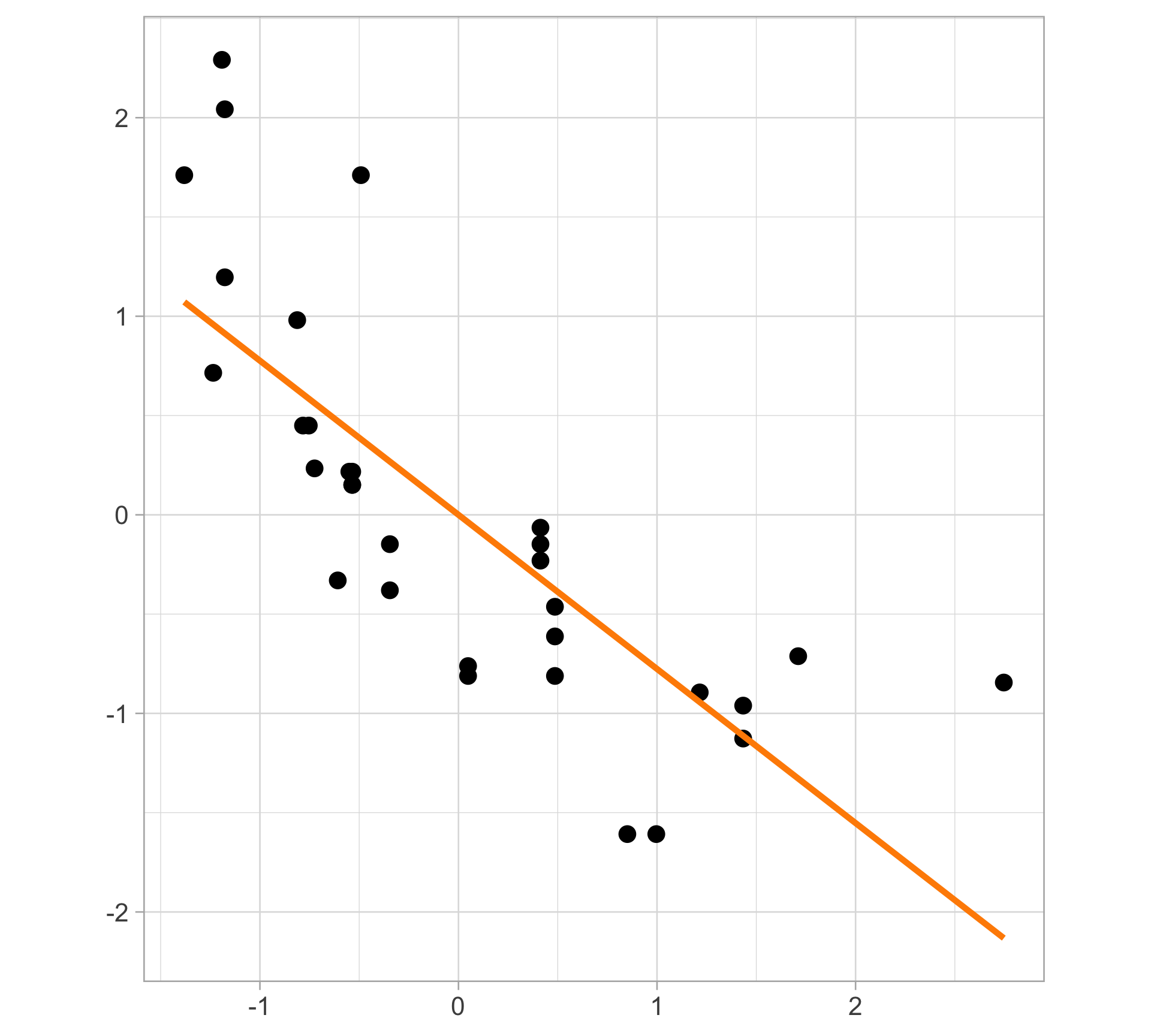
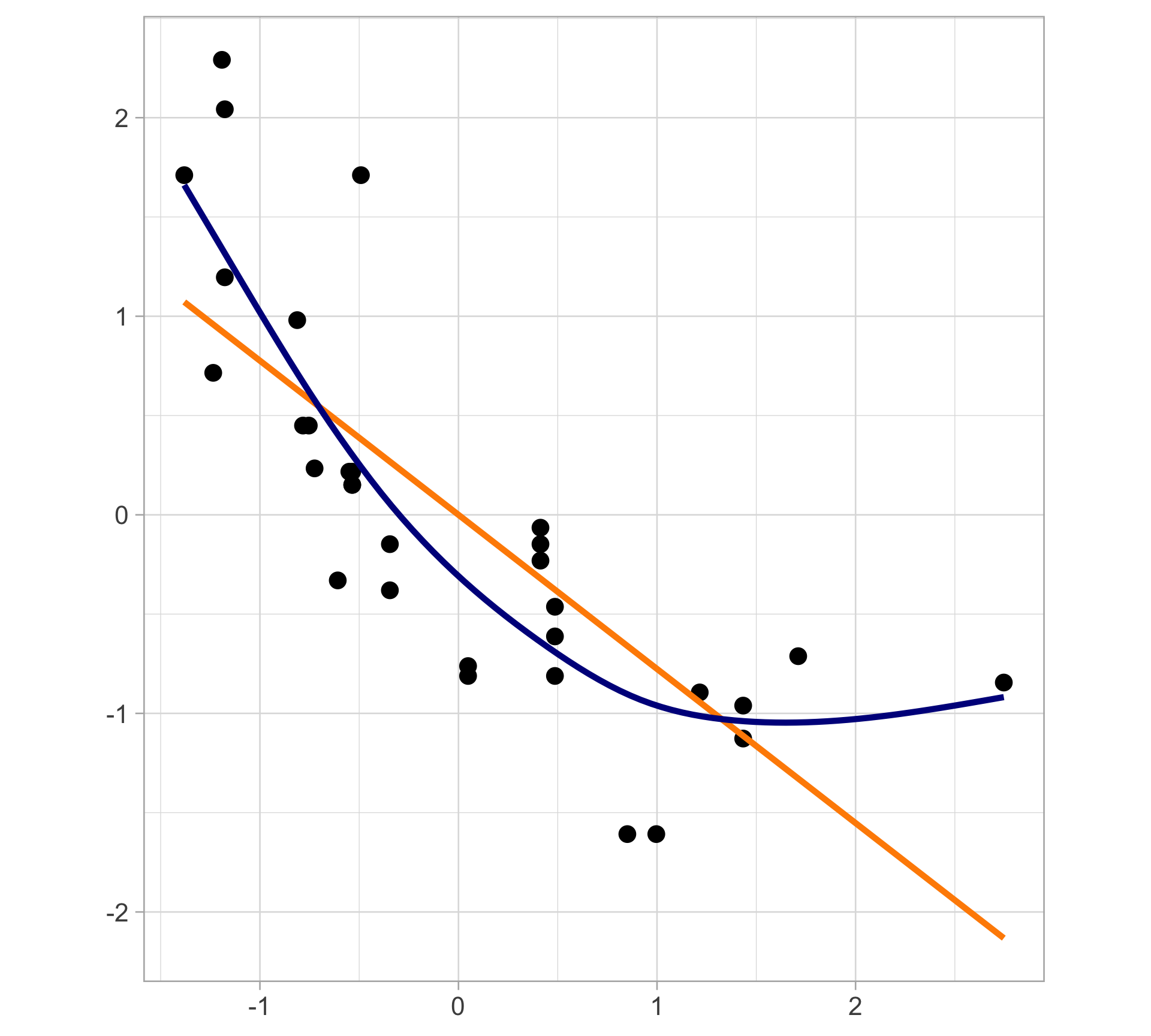
What if it’s not linear?
- Splines
- Local regression (LOESS)
- Generalized additive models (GAMs)
- Wavelets

The above methods can offer a lot of flexibility, without losing the ease and interpretability of linear models

Generalized additive models (GAMs)

Resources

Book: Generalized Additive Models by Simon Wood
GAM resources GitHub repository
mgcv workshop
Free GAM Course

Generalized additive models (GAMs)

Previously: generalized linear models (GLMs) (e.g., linear regression, logistic regression, Poisson regression)

GLM generalizes linear regression to permit non-normal distributions and link functions of the mean:

\[ g(\mathbb E[Y \mid X = x]) = \beta_0 + \beta_1 x_1 + \beta_2 x_2 + \dots + \beta_p x_p \]

What if we replace the linear predictor by additive smooth functions of the explanatory variables?

Entering generalized additive models (GAMs):

Relax the restriction that the relationship must be a simple weighted sum
Instead assume that the response can be modeled by a sum of arbitrary functions of each predictor

Generalized additive models (GAMs)

Allows for flexible nonlinearities in several variables

But retains the additive structure of linear models

\[g(\mathbb E[Y \mid X = x]) = \beta_0 + s_1(x_1) + s_2(x_2) + \dots + s_p(x_p)\]

Like GLMs, a GAM specifies a link function \(g()\) and a probability distribution for the response \(Y\)

\(s_j\) is some smooth function of predictor \(j\)

GLM is the special case of GAM in which each \(s_j\) is a linear function

Why use smooth functions?

Relationships between individual predictors and the response are smooth

Estimate the smooth relationships simultaneously to predict the response by adding them up

GAMs have the advantage over GLMs of greater flexibility (want to model the covariates flexibly, covariates and response not necessarily linearly related)

A disadvantage of GAMs/smoothing methods is the loss of interpretability: how do we interpret the effect of a predictor on the response?

Toy example: is this linear?

Toy example: linear regression fit

Toy example: GAM fit

Splines

A common way to smooth and learn nonlinear functions is to use splines

Splines can be used to approximate other, more complex functions

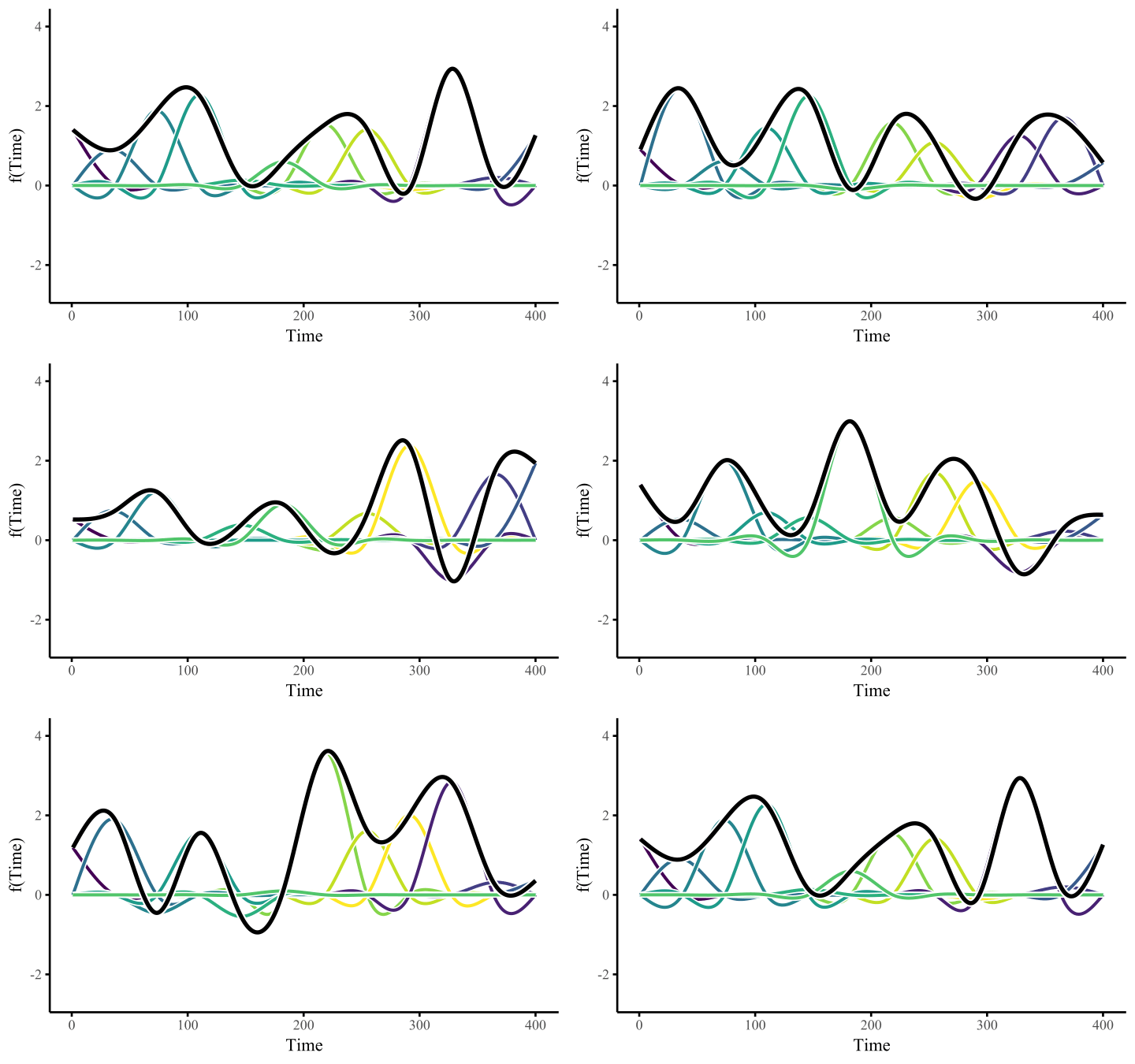
Splines are functions that are constructed from simpler basis functions (usually polynomials) . . .
Each basis function \(b_k\) has coefficient \(\beta_k\). Spline is just the sum of the weighted basis functions

\[\displaystyle s(x) = \sum_{k=1}^K \beta_k b_k(x)\]

Weight basis functions to obtain spline

Why not just a polynomial fit?

Suppose we are doing linear regression:

\[y_i \sim \mathcal{N}(\mu_i, \sigma^2)\] \[\mu_i = \beta_0 + \beta_1 x_{i} + \beta_2 x^2_{1i} + \cdots + \beta_j x^j_{i}\]

In the polynomial models we use a polynomial basis expansion of \(x\)
- \(x^0 = 1\) (constant term), \(x, x^2, x^3, x^4, \dots\)

We can keep on adding ever more powers of \(x\) to the model (hmm…)

Runge phenomenon: oscillations at the edges of an interval—using higher-order polynomials doesn’t always improve accuracy

Smoothing splines

Use smooth function \(s(x)\) to predict \(y\), control smoothness directly by minimizing the spline objective function

\[ \sum_{i=1}^n (y_i - s(x_i))^2 + \lambda \int s''(x)^2dx \]

\[= \text{fit data} + \text{impose smoothness}\]

\[\longrightarrow \text{model fit} = \text{likelihood} - \lambda \cdot \text{wiggliness}\]

Should remind you of penalized regression form!

Smoothing splines

The most commonly considered case: cubic smoothing splines

\[\text{minimize }\sum_{i=1}^n (y_i - s(x_i))^2 + \lambda \int s''(x)^2dx\]

First term: RSS, tries to make \(s(x)\) fit the data at each \(x_i\)

Second term: roughness penalty, controls how wiggly \(s(x)\) is via tuning parameter \(\lambda \ge 0\)
- Balances the accuracy of the fit and the flexibility of the function
- The smaller \(\lambda\), the more wiggly the function
- As \(\lambda \rightarrow \infty\), \(s(x)\) becomes linear

Smoothing splines

Goal: Estimate the smoothing spline \(\hat{s}(x)\) that balances the tradeoff between the model fit and wiggliness

Remember: Goldilocks principle

GAM recap

A framework to model flexible nonlinear relationships
Use little functions (basis functions) to make big functions
The predictor matrix has columns for each basis function, evaluated at each observation
Use a penalty term to trade off model fit and “wiggliness”
Need to make sure the smooths are wiggly enough without being overly wiggly

Example in `R`

Predicting MLB HR probability

Data available via the pybaseball library in python
Statcast data include pitch-level information, pulled from baseballsavant.com
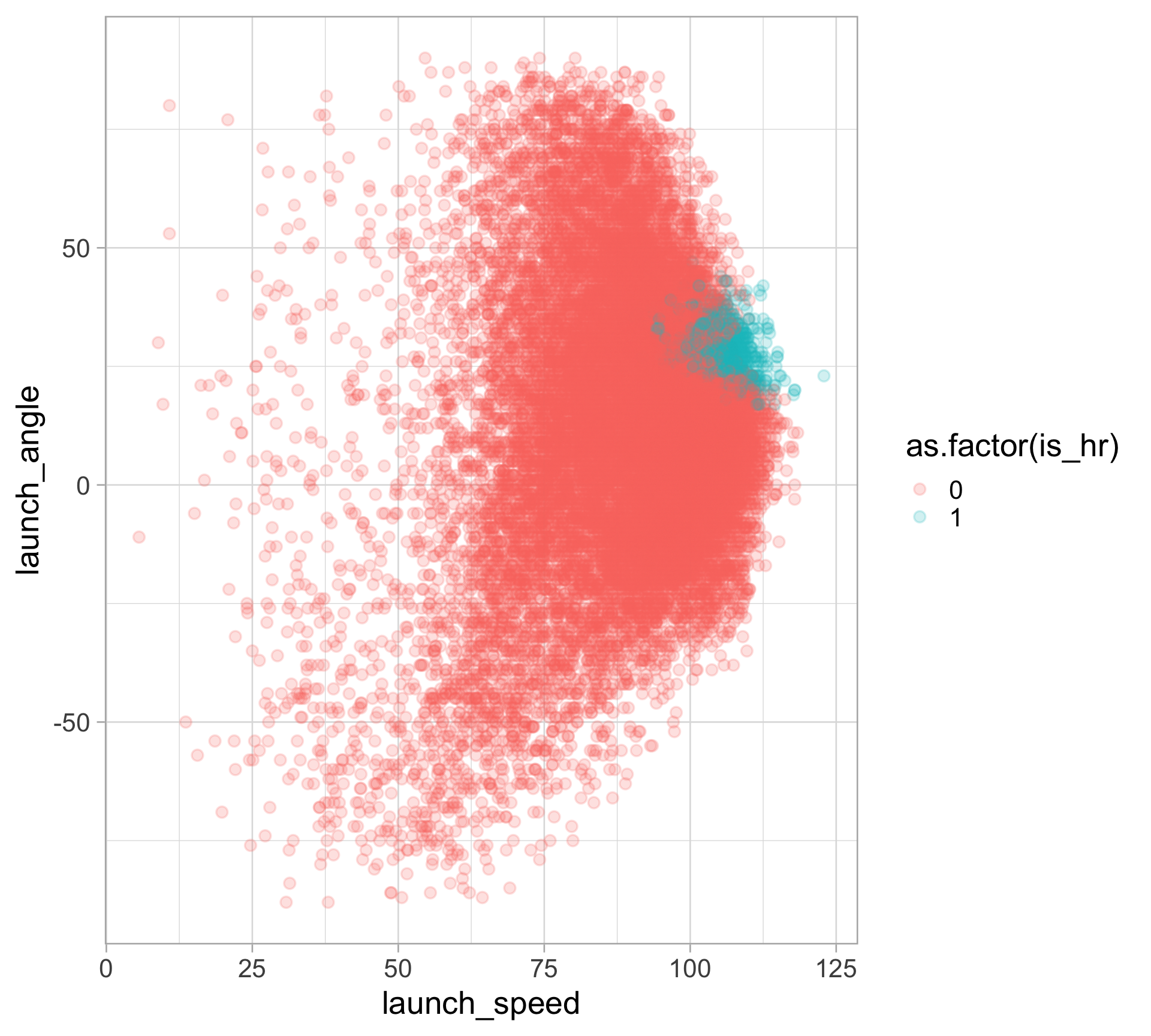
Example data collected for the entire month of May 2024

library(tidyverse)
savant <- read_csv("https://raw.githubusercontent.com/36-SURE/2026/main/data/savant.csv")
batted_balls <- savant |> 
  filter(type == "X") |> 
  mutate(is_hr = as.numeric(events == "home_run")) |> 
  filter(!is.na(launch_angle), !is.na(launch_speed), !is.na(is_hr))
# glimpse(batted_balls)

Predicting HRs with launch angle and exit velocity

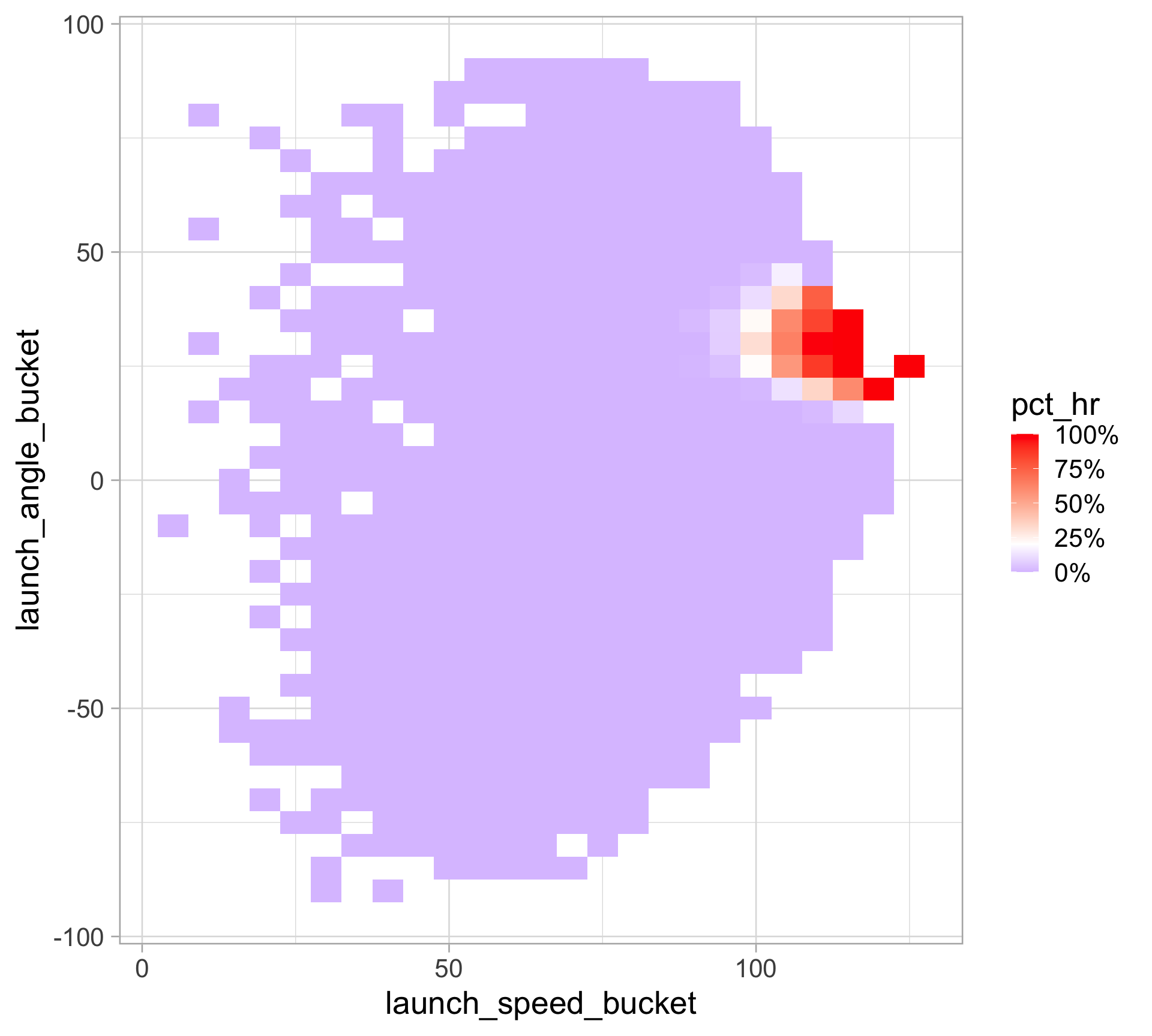
HRs are relatively rare and confined to one area of this plot

batted_balls |> 
  ggplot(aes(x = launch_speed, 
             y = launch_angle, 
             color = as.factor(is_hr))) +
  geom_point(alpha = 0.2)

Predicting HRs with launch angle and exit velocity

There is a sweet spot of launch_angle (mid-way ish) and launch_speed (relatively high) where almost all HRs occur

batted_balls |> 
  group_by(
    launch_angle_bucket = round(launch_angle * 2, -1) / 2,
    launch_speed_bucket = round(launch_speed * 2, -1) / 2
  ) |> 
  summarize(hr = sum(is_hr == 1),
            n = n()) |> 
  ungroup() |> 
  mutate(pct_hr = hr / n) |> 
  ggplot(aes(x = launch_speed_bucket, 
             y = launch_angle_bucket, 
             fill = pct_hr)) +
  geom_tile() +
  scale_fill_gradient2(labels = scales::percent_format(),
                       low = "blue", 
                       high = "red", 
                       midpoint = 0.2)

Fitting GAMs with mgcv

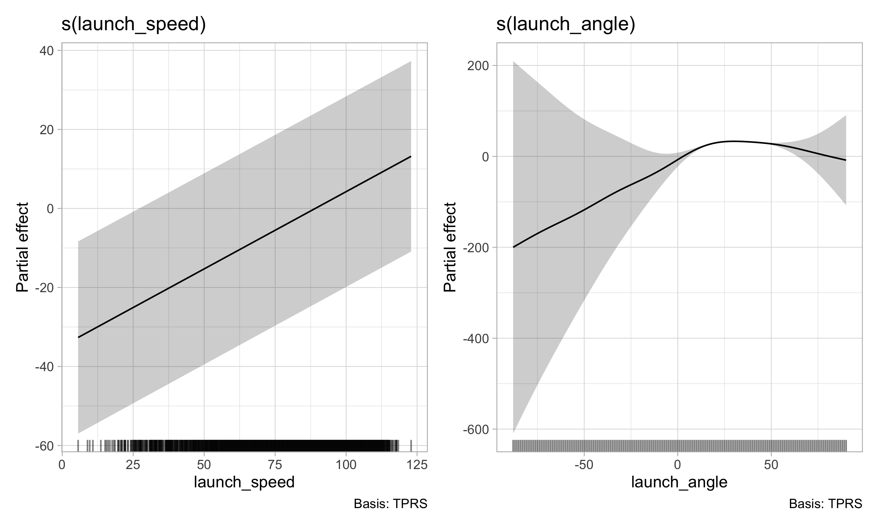
Modeling the log-odds of a home run using non-linear functions of launch_speed and launch_angle \[ \log \left( \frac{p_{\texttt{is_hr}}}{1 - p_\texttt{is_hr}} \right) = \beta_0 + s_1 (\texttt{launch_speed}) + s_2 (\texttt{launch_angle})\] where \(p_\texttt{is_hr}\) is the probability of a home run

Fit the model with smoothing spline functions s()

library(mgcv)
hr_gam <- gam(is_hr ~ s(launch_speed) + s(launch_angle),
              family = binomial,
              method = "REML", # more stable solution than default
              data = batted_balls)

View model summary

mgcv performs hypothesis tests for the smooth terms — these are roughly the equivalent of an \(F\)-test for dropping each term

Effective degrees of freedom (edf): basically the number of free parameters required to represent the function

In a smoothing spline, different choices of \(\lambda\) correspond to different values of the edf, representing different amounts of smoothness

library(broom)
tidy(hr_gam)

# A tibble: 2 × 5
  term              edf ref.df statistic p.value
  <chr>           <dbl>  <dbl>     <dbl>   <dbl>
1 s(launch_speed)  1.00   1.00      804.       0
2 s(launch_angle)  3.73   3.98      468.       0

tidy(hr_gam, parametric = TRUE)

# A tibble: 1 × 5
  term        estimate std.error statistic p.value
  <chr>          <dbl>     <dbl>     <dbl>   <dbl>
1 (Intercept)    -38.3      12.3     -3.11 0.00189

Visualize partial response functions

Display the partial effect of each term in the model and how they add up to the overall prediction

library(gratia)
draw(hr_gam)

To compare multiple models fit with gam(), we can also perform likelihood ratio (i.e., drop-in deviance) tests (via anova() from the mgcv package)

Model comparison: GAM vs GLM (logistic regression)

10-fold cross-validation: assigning games to folds

set.seed(25)
N_FOLDS <- 10
games_folds <- batted_balls |> 
  distinct(game_date, home_team, away_team) |>
  mutate(fold = sample(rep(1:N_FOLDS, length.out = n())))

batted_balls <- batted_balls |> 
  left_join(games_folds, by = join_by(game_date, home_team, away_team))

Cross-validation

hr_cv <- function(x) {
  hr_train <- batted_balls |> filter(fold != x)
  hr_test <- batted_balls |> filter(fold == x)
  
  gam_fit <- gam(is_hr ~ s(launch_speed) + s(launch_angle),
                 family = binomial,
                 method = "REML",
                 data = hr_train)
  logit_fit <- glm(is_hr ~ launch_speed + launch_angle, 
                   family = binomial, data = hr_train)
  
  hr_out <- tibble(
    gam_pred = predict(gam_fit, newdata = hr_test, type = "response"),
    logit_pred = predict(logit_fit, newdata = hr_test, type = "response"),
    test_actual = hr_test$is_hr,
    test_fold = x
  )
  return(hr_out)  
}

hr_preds <- map(1:N_FOLDS, hr_cv) |> 
  list_rbind()

Out-of-sample comparison

Very few situations in reality where GLMs (with a linear predictor) perform better than an additive model using smooth functions

Especially since smooth functions can just capture linear models

hr_preds |> 
  pivot_longer(cols = gam_pred:logit_pred, 
               names_to = "model", 
               values_to = "test_pred") |> 
  mutate(test_pred_class = round(test_pred)) |> 
  group_by(model, test_fold) |>
  summarize(accuracy = mean(test_pred_class == test_actual)) |> 
  group_by(model) |> 
  summarize(cv_accuracy = mean(accuracy),
            se_accuracy = sd(accuracy) / sqrt(N_FOLDS))

# A tibble: 2 × 3
  model      cv_accuracy se_accuracy
  <chr>            <dbl>       <dbl>
1 gam_pred         0.973     0.00105
2 logit_pred       0.959     0.00148

Appendix

Spline basis functions

Splines are piecewise cubic polynomials with knots (boundary points for functions) at every point

Practical alternative: linear combination of set of basis functions

Example: cubic polynomial

4 basis functions: \(B_1(x) = 1\), \(B_2(x) = x\), \(B_3(x) = x^2\), \(B_4(x) = x^3\)
\(\displaystyle r(x) = \sum_j^4 \beta_j B_j(x)\) is the regression function
Linear in the transformed variables \(B_1(x), \dots, B_4(x)\) but it is nonlinear in \(x\)

Extend this idea for splines piecewise using indicator functions so the spline is a weighted sum \[s(x) = \sum_j^m \beta_j B_j(x)\]

Number of spline basis functions

Think of the number of spline basis functions as a tuning parameter

Code to build dataset

# pip install pybaseball
# dictionary: https://baseballsavant.mlb.com/csv-docs
import pandas as pd
from pybaseball import statcast
savant = statcast(start_dt='2025-05-01', end_dt='2025-05-31')
savant.to_csv('savant.csv', index=False)

Supervised learning: nonparametric regression

Background

Recall: Model flexibility vs interpretability

\(k\)-nearest neighbors (\(k\)-NN)

Finding the optimal number of neighbors \(k\)

Moving beyond linearity

Generalized additive models (GAMs)

Generalized additive models (GAMs)

Generalized additive models (GAMs)

Why use smooth functions?

Toy example: is this linear?

Toy example: linear regression fit

Toy example: GAM fit

Splines

Weight basis functions to obtain spline

Why not just a polynomial fit?

Smoothing splines

Smoothing splines

Smoothing splines

GAM recap

Example in R

Predicting MLB HR probability

Predicting HRs with launch angle and exit velocity

Predicting HRs with launch angle and exit velocity

Fitting GAMs with mgcv

View model summary

Visualize partial response functions

Model comparison: GAM vs GLM (logistic regression)

Cross-validation

Out-of-sample comparison

Appendix

Spline basis functions

Number of spline basis functions

Code to build dataset

Example in `R`