Supervised learning: bagging and boosting


CMSACamp 2026

Department of Statistics & Data Science
Carnegie Mellon University

Decision trees review

Pros

  • Decision trees are very easy to explain and more closely mirror human decision-making

  • Easy to visualize and thus easy to interpret without assuming a parametric form

Cons

  • High variance: small changes in the input data can result in very different tree structures

  • Not often competitive in terms of predictive accuracy


We can combine multiple trees to improve accuracy (ensemble methods)

The bootstrap setup

The bootstrap is a fundamental resampling tool in statistics

Goal: quantify the uncertainty associated with a given estimator (e.g., obtain standard error, construct confidence intervals)

Setup: Given a sample \((X_1, Y_1), \dots, (X_n, Y_n)\) from an unknown distribution \(F\) (e.g., a normal distribution), and a statistic \(T\) (e.g., the mean) calculated from this sample

A bootstrap example

Task: estimate \(\textsf{Var}(T)\), where \(T\) is some statistic (like the sample mean)

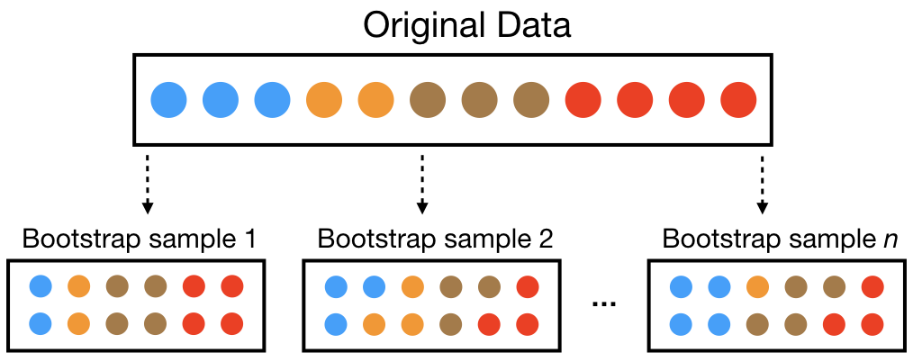
  1. Draw a bootstrap dataset of size \(n\) \((X_1^*, Y_1^*), (X_2^*, Y_2^*), \dots, (X_n^*, Y_n^*)\) by sampling \(n\) observations with replacement from the original data
  1. Compute the statistic of interest \(T\) on the bootstrapped dataset
  1. Repeat the previous two steps \(B\) times, to produce \(B\) bootstrap datasets and get \(T_1^*, T_2^*, \dots, T_B^*\)
  1. Obtain the variance estimate \(\displaystyle \widehat{\textsf{Var}}(T)\) as the sample variance of \(T_1^*, \dots, T_B^*\)


Note: not all of the original data points are represented in a bootstrap dataset, and some are represented more than once

Bagging

Bootstrap aggregation (bagging) is a general approach for reducing the variance of a statistical learning method

  • Bootstrap: take repeated samples with replacement from the training data
  • Aggregation: combine the results from many trees together, each constructed with a different bootstrapped sample of the data

Bagging algorithm

  • Construct \(B\) trees (e.g., \(B=1000\)) using \(B\) bootstrapped training sets, and average the resulting predictions
  • These trees are grown deep, and are not pruned (i.e. really overfitted)
  • Each individual tree has high variance, but low bias
  • Averaging these \(B\) trees reduces the variance

Bagging algorithm

To generate a prediction for a new observation:

  • Regression: take the average across the \(B\) trees

  • Classification: take the majority vote (most commonly occurring class) across the \(B\) trees

    • Could also use (average) probabilities instead…


The tradeoff with using bagging:

  • Improves prediction accuracy via wisdom of the crowds

  • But at the expense of interpretability (how do you read \(B = 1000\) trees?)

Out-of-bag (OOB) error

  • In bagging, the trees are constructed via bootstrapped data (sampling with replacement)
  • Each sample is likely to have duplicate observations

    • i.e. each tree is built only on a subset of the data that was sampled from the original data with replacement
  • On average, each bagged tree makes use of around 2/3 of the observations

Why? Hint: The probability of a specific observation never gets selected in any of the \(B\) draws is \((1-1/B)^B\)

  • The remaining observations not used to fit a given bagged tree are referred to as the out-of-bag (OOB) observations
  • We can use the OOB samples to estimate predictive performance

Random forests

TL;DR: Random forests are bagged trees except that we also choose random subsets of predictors for each tree

  • Random forests provide an improvement over bagged trees with a small tweak that decorrelates the trees

    • This reduces the variance when we average the trees
  • As in bagging, we build a number of decision trees on bootstrapped training samples
  • But we only consider a random subset of \(m\) predictors (from the full set of \(p\) predictors) at each potential split

    • The split is allowed to use only one of those \(m\) predictors

    • This adds more randomness to make each tree more independent of each other

  • \(m\) is a tuning parameter — typically use \(m = p/3\) (regression) or \(m = \sqrt{p}\) (classification)

Random forests

See also: this joke

Example: 2022 Men’s FIFA World Cup shots

Goal: predict whether the shot was a goal using shot-level attributes

library(tidyverse)
theme_set(theme_light())

mwc_shots <- read_csv("https://raw.githubusercontent.com/36-SURE/2026/main/data/mwc_shots.csv")
head(mwc_shots)
# A tibble: 6 × 34
   ...1 possession_team_name player_name     position_name player_name_gk period
  <dbl> <chr>                <chr>           <chr>         <chr>           <dbl>
1     1 Tunisia              Youssef Msakni  Left Wing     Kasper Schmei…      1
2     2 Tunisia              Issam Jebali    Center Forwa… Kasper Schmei…      1
3     3 Tunisia              Mohamed Dräger  Right Wing B… Kasper Schmei…      1
4     4 Tunisia              Youssef Msakni  Left Wing     Kasper Schmei…      1
5     5 Denmark              Kasper Dolberg  Left Center … Aymen Dahmen        1
6     6 Denmark              Joachim Anders… Right Center… Aymen Dahmen        1
# ℹ 28 more variables: minute <dbl>, second <dbl>, duration <dbl>,
#   under_pressure <lgl>, play_pattern_name <chr>, shot_technique_name <chr>,
#   shot_body_part_name <chr>, shot_outcome_name <chr>, location_x <dbl>,
#   location_y <dbl>, location_x_gk <dbl>, location_y_gk <dbl>,
#   dist_to_goal <dbl>, dist_to_keeper <dbl>, angle_to_goal <dbl>,
#   angle_to_keeper <dbl>, angle_deviation <dbl>, avevelocity <dbl>,
#   dist_sgk <dbl>, density_incone <dbl>, attackers_behind_ball <dbl>, …

Example using ranger

ranger package provides a fast implementation of random forests in R

Fitting a plain random forest model with no tuning

library(ranger) # install.packages("ranger")
set.seed(0630)
# prop.table(table(mwc_shots$goal))
mwc_shots_rf <- ranger(goal ~ location_x + location_y + angle_to_goal + play_pattern_name 
                       + avevelocity + angle_to_keeper + dist_to_keeper + density_incone,
                       num.trees = 500, importance = "impurity", data = mwc_shots,
                       probability = TRUE)
# mwc_shots_rf

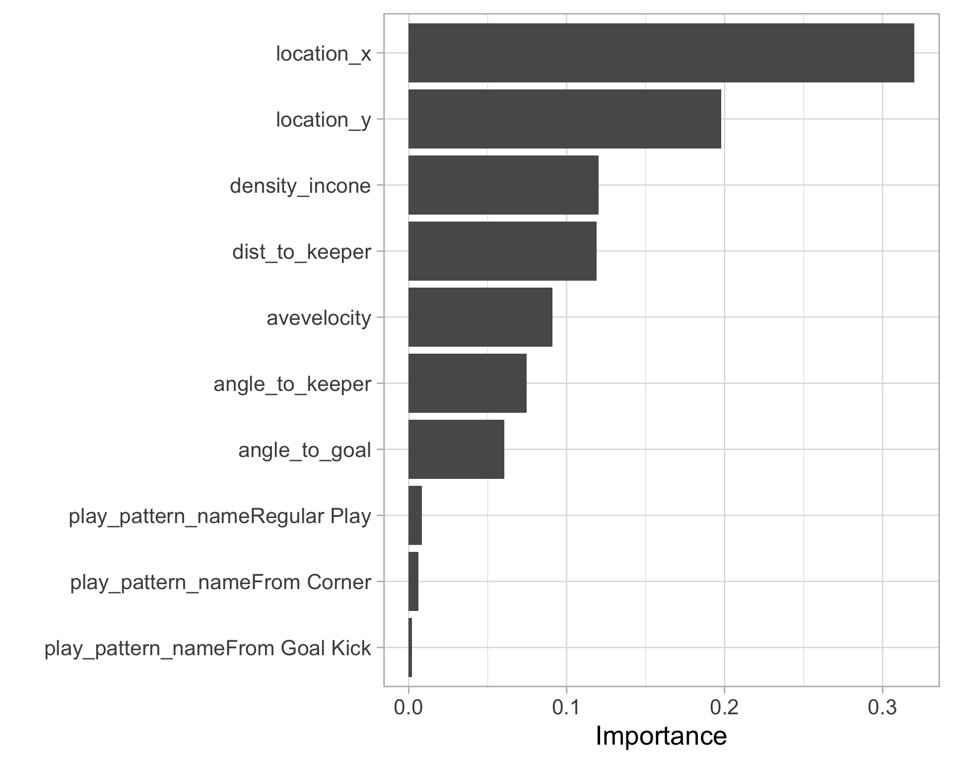
Variable importance

There are two popular ways to measure variable importance for random forests:

  1. For each variable, measure the amount that RSS (or Gini index) decreases
    due to splits in that variable. Average this over all trees in the forest

  2. Randomly permute each variable (one at a time) and see how much
    the model performance decreases

library(vip)
vip(mwc_shots_rf)

Model evaluation

  1. Brier score
#mwc_shots_rf$prediction.error
mwc_shots |> 
  mutate(goal_prob = mwc_shots_rf$predictions[,"1"]) |> 
  summarize(briar_score = mean((goal_prob - goal)^2))
# A tibble: 1 × 1
  briar_score
        <dbl>
1      0.0834
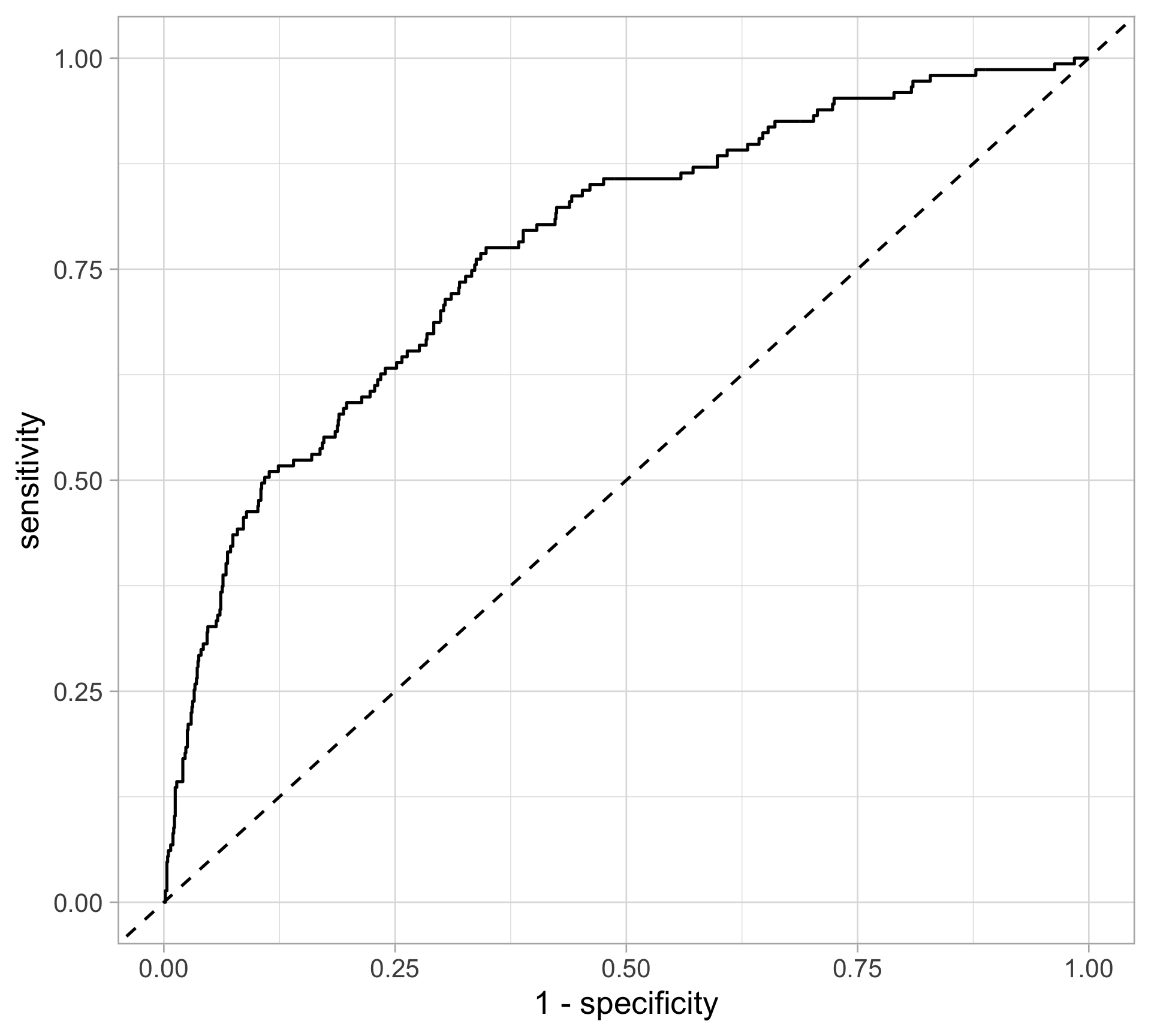
  1. Calculate the AUC and plot the ROC curve
library(pROC)
mwc_shots_rfroc <- mwc_shots |> 
  mutate(goal_prob = mwc_shots_rf$predictions[,"1"]) |> 
  roc(goal, goal_prob)
  
mwc_shots_rfroc$auc
Area under the curve: 0.7744
rf_roc <- tibble(threshold = mwc_shots_rfroc$thresholds,
       specificity = mwc_shots_rfroc$specificities,
       sensitivity = mwc_shots_rfroc$sensitivities) 
rf_roc |> 
  ggplot(aes(x = 1 - specificity, y = sensitivity)) +
  geom_path() +
  geom_abline(slope = 1, intercept = 0, 
              linetype = "dashed")

Tuning random forests

Number of trees

  • It is more efficient to just pick a large enough value (e.g., 1000 trees) instead of tuning this

  • No risk of overfitting if we pick something too big

NOTE: The important parameter to tune is mtry (number of predictors at each split)

  • The default (\(p/3\) (regression) or \(\sqrt{p}\) (classification)) often does a good job


Check out Julia Silge’s tutorials on using tidymodels to tune random forests (and other ML models)

Boosting

Bagging (and random forests) is a parallel ensemble model

  • Create multiple copies of the original training data set using the bootstrap

  • Fit a separate decision tree to each copy

  • Combine all of the trees in order to create a single predictive model

  • Important takeaway: each tree is built on a bootstrap data set, independent of the other trees

Boosting is a sequential ensemble model

  • Trees are grown sequentially (using the entire training dataset)

  • Each tree is grown using information from previously grown trees

Boosting

Builds ensemble models sequentially

  • Start with a weak learner (e.g., a small decision tree with few splits, or even the simplest version: a decision stump, i.e. a decision tree with just one node)
  • Each model in the sequence slightly improves upon the predictions of the previous models by focusing on the observations with the largest residuals

Intuition behind boosting

  • Instead of fitting a single large decision tree, which could result in overfitting, boosting learns slowly
  • Given the current model, we fit a decision tree to the residuals from the model
  • We then add this new decision tree into the fitted function in order to update the residuals
  • Each of these trees can be rather small, with just a few terminal nodes (this is a tuning parameter)
  • The goal of fitting small trees to the residuals is to slowly improve the model fit in areas where it does not perform well
  • Incorporate a shrinkage parameter (i.e. learning rate) which slows the process down, which reduces the risk of overfitting but increases training time

Boosting: more details

  • Given training data \((x_i, y_i), \ i = 1, \dots, n\)
  • We’ll focus on classification and assume \(y_i \in \{-1, 1\}\)
  • Suppose that a classification tree (fit, e.g., to the training data) will return a prediction of the form \(\hat f^\text{tree}(x) \in \{-1, 1\}\) for an input \(x\)
  • In boosting we combine a weighted sum of \(B\) different tree classifiers \(\displaystyle \hat f ^\text{boost} (x) = \text{sign} \left\{\sum_{b=1}^B \alpha_b \hat f^{\text{tree},b}(x)\right\}\)
  • One of the key differences between boosting and bagging is how the individual classifiers \(\hat f^{\text{tree},b}\) are fit
  • In boosting we fit the tree to the entire training dataset, and adaptively weight the observations to encourage better predictions for points that were previously misclassified

Basic boosting algorithm (AdaBoost)

Given training data \((x_i, y_i), \ i = 1, \dots, n\)

  • Initialize the weights by \(w_i = 1/n\) for each \(i\)
  • For \(b = 1, \dots, B\):

    • Fit a classification tree \(\hat f^{\text{tree},b}\) to the training data with weights \(w_1, \dots, w_n\)

    • Compute the weighted misclassification error \(\displaystyle e_b = \frac{\sum_{i=1}^n w_i I\{y_i \ne \hat f^{\text{tree},b} (x_i)\}}{\sum_{i=1}^n w_i}\)

    • Let \(\displaystyle \alpha_b = \log \frac{1 - e_b}{e_b}\)

    • Update the weights as \(w_i \leftarrow w_i \cdot \exp\{\alpha_b I\{y_i \ne \hat f^{\text{tree},b} (x_i)\} \}\)

  • Return \(\displaystyle \hat f ^\text{boost} (x) = \text{sign} \left\{\sum_{b=1}^B \alpha_b \hat f^{\text{tree},b}(x)\right\}\)

Why does boosting work?

  • Simple intution: weight misclassified observations in such a way that
    they get properly classified in future iterations
  • Boosting essentially fits an additive model as a function of trees \(T_1(x_i), \dots, T_M(x_i)\)
  • For classification, use the exponential loss \(\exp(-y_if(x_i))\)
  • Use a forward stepwise procedure (similar to forward stepwise regression)

    • Choose the tree \(T_j\) and weight \(\beta_j\) giving the smallest exponential loss \(\displaystyle \sum_{i=1}^n \exp\{-y_i \beta_j T_j (x_i)\}\)

    • Choose the tree \(T_j\) and weight \(\beta_j\) giving the smallest additional loss \(\displaystyle \sum_{i=1}^n \exp\{-y_i \{\beta_j T_j (x_i) + \beta_k T_k (x_i)\}\}\)

    • Repeat the last step

Variable importance for boosting

  • For a single decision tree \(\hat f^{\text{tree}}\), define the squared importance for variable \(j\) as

\[\text{Imp}^2_j \left(\hat f ^\text{tree}\right) = \sum_{k=1}^m \hat d_k \cdot I \{\text{split at node } k \text{ is on variable } j\}\]

where \(m\) is the number of internal nodes and \(\hat d_k\) is the improvement in training misclassification error from making the \(k\)-th split

  • For boosting, define the squared importance for a variable \(j\) by simply averaging the squared importance over all of the fitted trees

\[\text{Imp}^2_j \left(\hat f ^\text{boost}\right) = \frac{1}{B} \sum_{i=1}^B f ^ {\text{tree}, b}\]

  • We usually consider the largest importance value and scale all of the other variable importances accordingly, which are then called relative importances

Gradient boosted trees

  • Boosting can be generalized to other loss functions via gradient descent
  • Entering gradient boosted trees, or gradient boosting machines (GBMs)
  • Update the model parameters in the direction of the loss function’s descending gradient

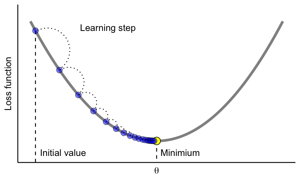
Gradient descent

  • Let \(\theta\) denote the vector of all parameters

  • Let \(\ell(\theta, D)\) denote the loss function for \(n\) data points \(D_i\)


Main idea: Start with an initial guess for \(\theta\), then iterate until the loss function fails to decrease

  • Tuning parameter: learning rate \(\eta\)
  • Intuition: move a small step downhill based on the gradient at current position

\[\theta_t \leftarrow \theta_{t-1} - \eta \nabla_\theta \ell(\theta, D) \vert _{\theta = \theta_{t-1}}\]

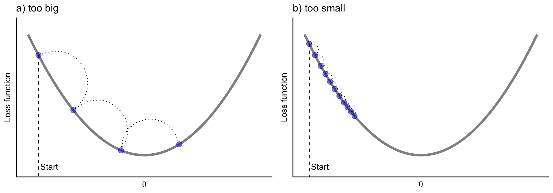
Tune the learning rate in gradient descent

We need to control how much we update by in each step: the learning rate

Stochastic gradient descent (SGD)

  • Gradient descent requires computing over entire dataset at each iteration

    • Usually takes many steps to reach a local minimum.

    • Computationally prohibitive for massive sample sizes

    • Complicated models need to be optimized for many iterations

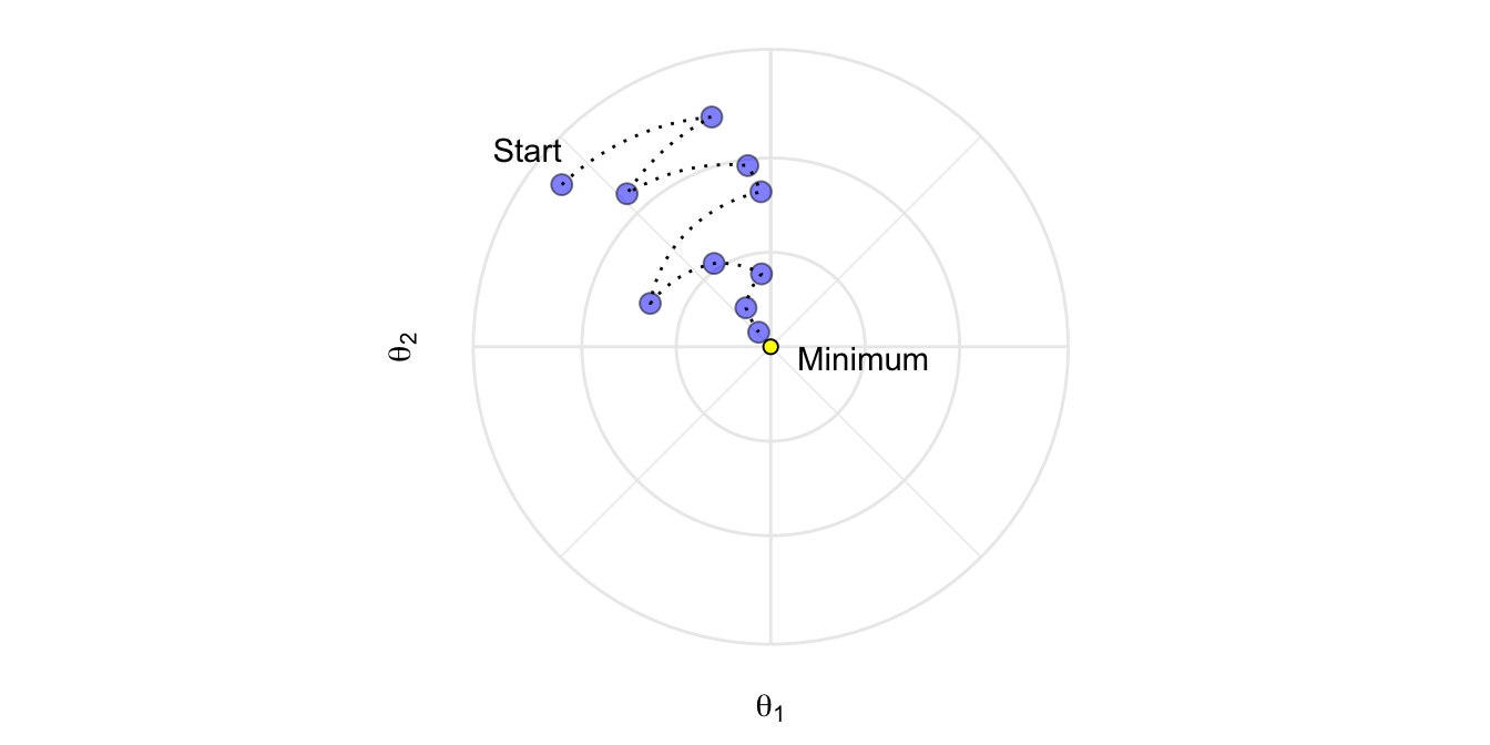
  • Stochastic gradient descent (SGD): sample a small fraction (minibatch) of the data to compute a gradient step

SGD can help with complex loss functions

  • Speed up algorithm while adding randomness to get closer to global minimum (no guarantees!)

  • Much less smooth due to its random nature

  • The path (ensemble of intermediate parameter values) toward the minimum will be zigzaggy

Extreme gradient boosting with XGBoost

XGBoost (eXtreme Gradient Boosting) is an efficient, flexible, and portable boosting library . . .

XGBoost hyperparameters for tuning

  • Number of trees \(B\) (nrounds)

  • Learning rate (eta), i.e. how much we update in each step

    • Note: these two really have to be tuned together
  • Complexity of the trees (depth, number of observations in nodes)
  • Regularization (gamma) and early stopping

For more details on the hyperparameters for tuning, see the XGBoost Parameters page

Be responsible!

XGBoost is more flexible, but requires more work to tune properly as compared to random forests

XGBoost example: Preprocessing data

First, we select our predictor columns and create a xgb.DMatrix object

library(xgboost)

x_train <- mwc_shots |> 
  select(location_x, location_y, angle_to_goal, play_pattern_name,
         avevelocity, angle_to_keeper, dist_to_keeper, density_incone) 

dtrain <- xgb.DMatrix(data = model.matrix(~ . - 1, data = x_train),
                      label = as.numeric(mwc_shots$goal == 1))

XGBoost example: Cross validation

Next, we define all combinations of parameters we are interested in

# Define a grid of hyperparameters
xg_grid <- expand.grid(
  nrounds = seq(20, 150, 10),
  max_depth = c(2, 3, 4),
  eta = c(0.01, 0.05, 0.1),
  gamma = 0,
  colsample_bytree = 1,
  min_child_weight = 1,
  subsample = 1
)

XGBoost example: Cross validation

After, we map over all combinations and do 5-fold cross validation

library(purrr)

cv_results <- map(1:nrow(xg_grid), function(i) {
  params <- list(
    objective = "binary:logistic",
    eval_metric = "auc", # cv metric 
    max_depth = xg_grid$max_depth[i],
    eta = xg_grid$eta[i],
    gamma = xg_grid$gamma[i],
    colsample_bytree = xg_grid$colsample_bytree[i],
    min_child_weight = xg_grid$min_child_weight[i],
    subsample = xg_grid$subsample[i]
  )
  # Run CV for the current parameter set
  cv <- xgb.cv(
    params = params,
    data = dtrain,
    nfold = 5,
    # how many boosting rounds
    nrounds = xg_grid$nrounds[i],
    maximize = TRUE, # want to maximize cv metric (since auc) 
    verbose = FALSE,
  )
  
return(list(params = params,
            nrounds = xg_grid$nrounds[i],
            best_auc = max(cv$evaluation_log$test_auc_mean)))
})

XGBoost example: Fitting the model

From here, we can find the best overall configuration (aka the one that gives us the maximum AUC)

best_result <- cv_results[[which.max(purrr::map_dbl(cv_results, "best_auc"))]]
# print(best_result)

Finally, we can fit our xgboost model (yay!)

xg_fit <- xgb.train(
  params = best_result$params,
  data = dtrain, # ideally, we would use new data (completely unseen)
  nrounds = best_result$nrounds,
  verbose = FALSE
)

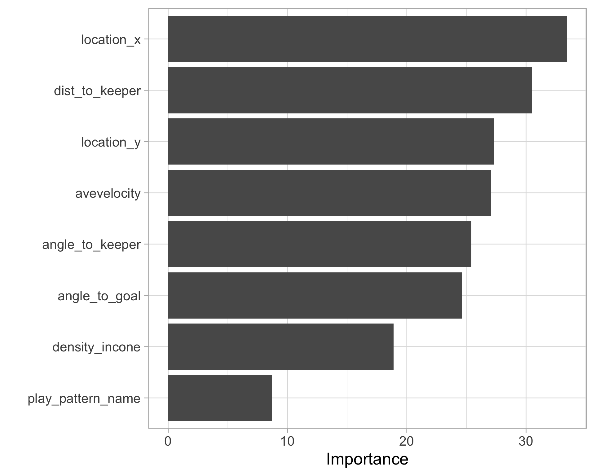
Variable importance and model evaluation

library(vip)
xg_fit |> 
  vip()

  1. Brier score
mwc_shots |> 
  mutate(goal_prob = predict(xg_fit, newdata = dtrain, type = "response")) |> 
  summarize(briar_score = mean((goal_prob - goal)^2))
# A tibble: 1 × 1
  briar_score
        <dbl>
1      0.0615
  1. AUC
mwc_shots_xgroc <- mwc_shots |> 
  mutate(goal_prob = predict(xg_fit, newdata = dtrain, type = "response")) |> 
  roc(goal, goal_prob)

mwc_shots_xgroc$auc
Area under the curve: 0.9284

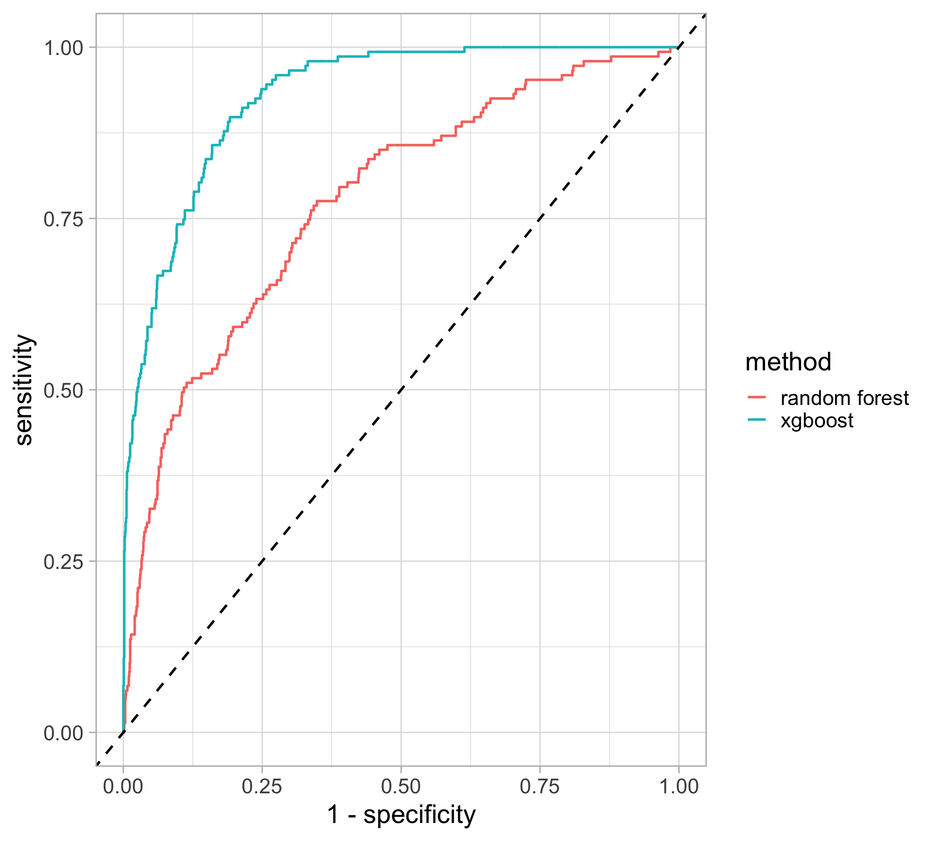
Comparing random forest and xgboost models

Note: this is only a rough comparison…ideas for why?

tibble(threshold = c(mwc_shots_xgroc$thresholds),
       specificity = mwc_shots_xgroc$specificities,
       sensitivity = mwc_shots_xgroc$sensitivities,
       method = "xgboost") |> 
  rbind(mutate(rf_roc, method = "random forest")) |>
  ggplot(aes(x = 1 - specificity, y = sensitivity, color = method)) +
  geom_path() +
  geom_abline(slope = 1, intercept = 0, 
              linetype = "dashed") 

See also

Appendix: creating the dataset with StatBombR

library(tidyverse)
library(StatsBombR)

mwc <- FreeCompetitions() |> 
  filter(competition_id == "43" & season_id == "106") |> 
  FreeMatches() |> 
  free_allevents() |> 
  allclean()

mwc_shots <- mwc |>
  filter(type.name == "Shot", 
         shot.type.name == "Open Play", 
         team.name == possession_team.name) |> 
  janitor::remove_empty() |> 
  select(possession_team.name, player.name, position.name, player.name.GK,
         period, minute, second, duration, under_pressure, 
         play_pattern.name, shot.technique.name, shot.body_part.name, shot.outcome.name,
         location.x, location.y, location.x.GK, location.y.GK, 
         DistToGoal, DistToKeeper, AngleToGoal,AngleToKeeper, AngleDeviation, 
         avevelocity, DistSGK, density.incone, 
         AttackersBehindBall:InCone.GK, TimeInPoss, TimeToPossEnd) |> 
  mutate(InCone.GK = ifelse(InCone.GK > 0, 1, InCone.GK),
         under_pressure = if_else(is.na(under_pressure), FALSE, under_pressure),
         goal = as.factor(if_else(shot.outcome.name == "Goal", 1, 0))) |>
  janitor::clean_names()
Appendix: tuning XGBoost with caret

library(caret)

# create hyperparameter grid
xg_grid <- crossing(nrounds = seq(20, 150, 10),
                    eta = c(0.01, 0.05, 0.1), gamma = 0,
                    max_depth = c(2, 3, 4), colsample_bytree = 1,
                    min_child_weight = 1, subsample = 1)


# tuning
xg_tune <- train(x = x_train,
                 y = as.factor(mwc_shots$goal), 
                 tuneGrid = xg_grid,
                 trControl = trainControl(method = "cv", number = 5),
                 objective = "binary:logistic", 
                 method = "xgbTree")

# fit final model  data
xg_fit <- xgboost(
  data = x_train,
  label = as.factor(mwc_shots$goal),
  objective = "binary:logistic",
  nrounds = xg_tune$bestTune$nrounds,
  params = as.list(select(xg_tune$bestTune, -nrounds)),
  verbose = 0
)

Appendix: Statistics or Machine Learning?