Advanced topics: survival analysis

CMSACamp 2026

Department of Statistics & Data Science
Carnegie Mellon University

Background

Motivation

Previously:

• Considered problems of the form: “model the relationship between \(X\) and \(Y\)”, where:

  • \(X\) and \(Y\) are completely observed

  • Make assumptions about the distribution of \(Y\) and the shape of the relationship

• Example: use game- and shot-level features to predict goal probability

But not every statistical problem is of this form!

Suppose we want to model the time-to-event, where:

• That time might be incompletely observed for certain observations/units (\(Y\) is not completely observed)

• Each observation/unit can experience a certain event a maximum of one time

The field of survival analysis is about modeling time-to-event outcomes!

Examples of time-to-event outcomes

• Time until injury

• Time until an athlete transfers

• Time until death

• Time until a patient is discharged from the hospital

• Time until a user cancels a subscription service

• Time until a convicted criminal reoffends

• Time until a PhD student graduates

In survival analysis:

• We are interested in modeling the rate of the event-of-interest (not just if the event happened)

• Generically, we call the event-of-interest failure (or death), i.e, we are interested in modeling failure (death) rates and risk of failure (death) for each observation

Two possible outcomes

Suppose observe each observation \(i\) beginning at time zero. For each observation \(i\), there are two possible outcomes:

1. The observation “fails” (aka has the event occur) at time \(T_i\). This is known as the failure time or the survival time (since that is how long the observation survives)

2. The observation reaches time \(C_i\) without failure (aka without the event occurring), and no longer observe the observation after that time to know when the event occurs

Case 2 is called censoring because the true time-to-event \(T_i\) is censored or unknown to us — all we know is that \(T_i > C_i\)

Technically, we focus on right-censoring, which is when we only know that \(T_i > C_i\).¹

1. There are other types of censoring, such as left-censoring (where \(T_i < C_i\)) and interval censoring (where \(T_i \in [c_{i1}, c_{i2}]\)).

So basically…

Fundamental challenge: censoring

• Censoring can happen for various reasons:

  • Example 1: a player leaves a team for financial reasons

  • Example 2: a player leaves a team because of recurring minor injuries or reduced fitness

• Censoring is effectively a missing data problem since we are missing the true time-to-event (outcome)

So, why not just do a complete case analysis, where we filter out censored observations?

• Filtering out censored observations is problematic for two reasons:

  • It throws away useful information: we lose useful information that they survived up until time \(C_i\)

  • It can bias analysis: an observation may be censored for reasons that are related to the event-of-interest (aka it may be informative)

Survival analysis problem setup

In survival analysis, we are interested in modeling \(T_i\) while accounting for censoring

Data: Suppose we have \(n\) i.i.d observations of the following form:

\[(\mathbf{X}_1, Y_1, R_1), \dots, (\mathbf{X}_n, Y_n, R_n)\] where:

• \(\mathbf{X}_i\): feature vector for unit \(i\) (e.g., age, position, minutes player)

• \(Y_i\): either the observed time-to-event \(T_i\) or the censoring time \(C_i\) depending on what happened first (\(Y_i = \min\{T_i, C_i\}\))

• \(R_i\): status of whether the event-of-interest occurred

\[ R_i = \begin{cases} 1 \quad \text{if } Y_i = T_i, \\ 0 \quad \text{if } Y_i = C_i \end{cases} \]

Survival function

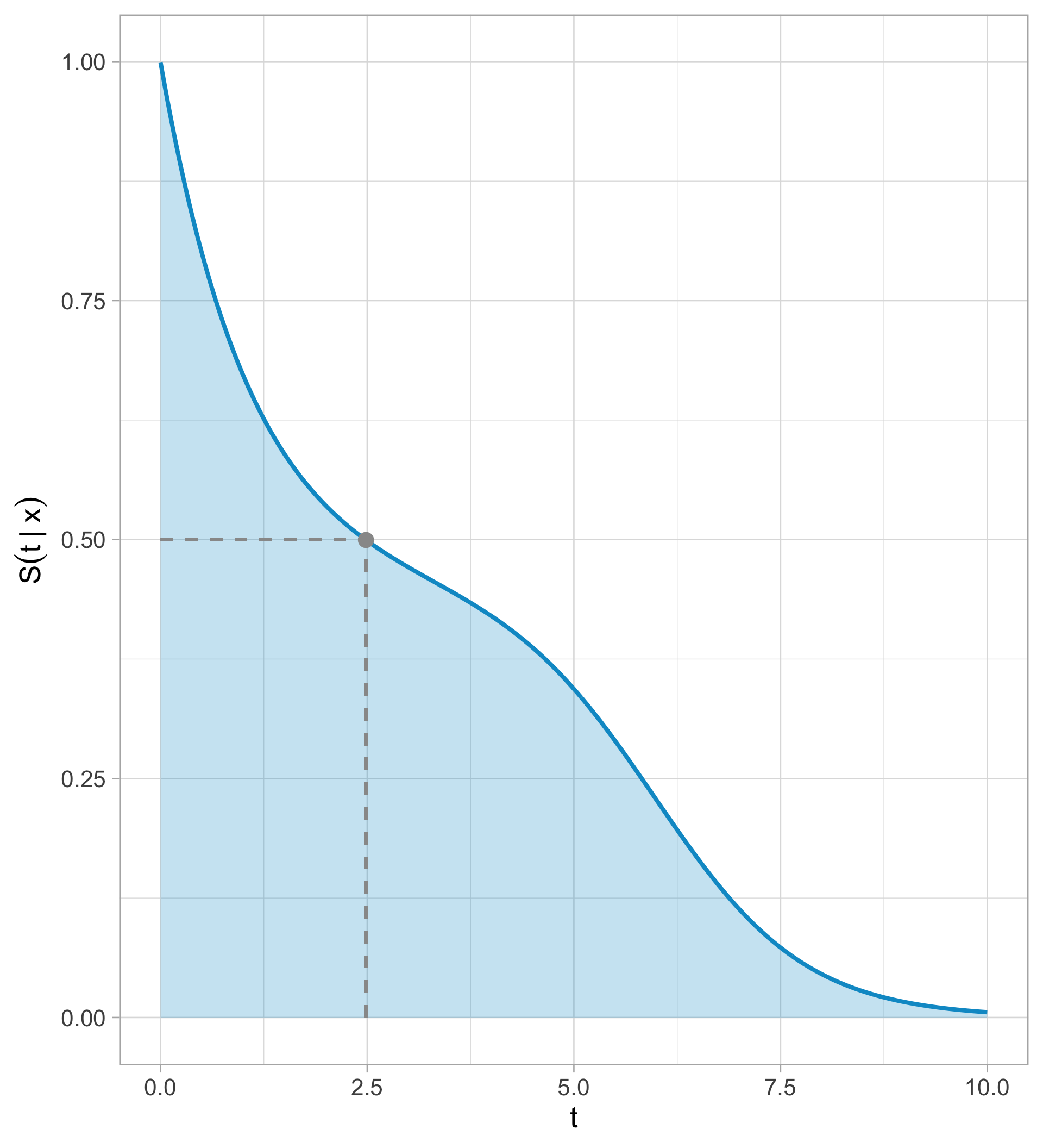
The survival function is defined as follows:

\[ S(t \mid \mathbf{x}) := \displaystyle \text{Pr}(T > t \mid \mathbf{x}) = \text{Pr}(\text{survive beyond time } t \mid \mathbf{x}) \]

Note:

• If we start observing every unit \(i\) at \(t = 0\), then \(S(0 \mid \mathbf{x}) = 1\)

• \(S(t \mid x)\) declines as \(t \to \infty\):

  • For some events-of-interest that will necessarily happen (e.g., death): \(S(t \mid \mathbf{x}) \to 0\) as \(t \to \infty\)

  • For others events-of-interest where the event does not necessarily happen (e.g., injury): \(S(t \mid \mathbf{x})\) declines to some positive value (between zero and one) as \(t \to \infty\)

• We are predicting whole curves per feature vector \(\mathbf{x}\), not just a single value!

Interpreting the survival curve

What the time-to-event outcome is matters for our interpretation:

• For time until injury, longer is considered “better”

• For time until a patient is discharged, longer is often considered “worse”

From the survival curve:

• The median survival time of \(\mathbf{x}\) is where \(S(t \mid \mathbf{x}) = 1/2\)

• The mean survival time of \(\mathbf{x}\) is the area under the survival curve: \(\displaystyle \int_0^\infty S(t \mid \mathbf{x}) dt\)

Kaplan-Meier curves

Kaplan-Meier curves are a popular estimator of survival curves

Let’s ignore the feature vector for now, so that our data is of the form: \((Y_1, R_1), \dots (Y_n, R_n)\)

First, we find all unique observed times in which event-of-interest occurred

\[ 0 < \tau_{(1)} < \tau_{(2)} < \dots < \tau_{(L)}, \qquad L = \text{# of unique event times} \]

Let:

• \(n[m]\) denote number of observations that are “at risk” right before time \(\tau_{(m)}\)

• \(d[m]\) denote the number of observations that “die” at time \(\tau_{(m)}\)

Kaplan-Meier curves

For observations “at risk” at the beginning of time \(\tau_{(m)}\), the probability of surviving that time is:

\[ p_m = \frac{n[m] - d[m]}{n[m] } \]

E.g., the probability that an observation survives to the second time \(\tau_{(2)}\), given they survived the first time \(\tau_{(1)}\) is:

\[ p_2 = \frac{n[2] - d[2]}{n[2]} \]

The probability that (at the outset) an observation survives to the second time \(\tau_{(2)}\) is:

\[ \begin{aligned} \text{Pr}(T > \tau_{(2)}) &= \text{Pr}(T > \tau_{(1)}) \cdot \text{Pr}(T > \tau_{(2)} \mid T > \tau_{(1)}) = \frac{n[1] - d[1]}{n[1]} \cdot \frac{n[2] - d[2]}{n[2]} = p_1 \cdot p_2 \end{aligned} \]

Kaplan-Meier curves

Therefore, the Kaplan-Meier estimate for the probability of surviving the first \(t\) days is:

\[ \hat{S}(t)_{\text{KM}} = \prod_{m = 1, \dots, L \text{ s.t. } \tau_{(m)} \leq t} \frac{n[m] - d[m]}{n[m]} = \prod_{m = 1, \dots, L \text{ s.t. } \tau_{(m)} < t} p_m \]

• The Kaplan-Meier curve is a non-parametric estimator of the survival function — doesn’t assume a parametric form!

• We can derive point-wise confidence intervals for Kaplan-Meier curves

• There are extensions that allow us to add in feature vectors, i.e., that estimate \(S(t \mid \mathbf{x})\) using \(k\) nearest neighbor or kernel approaches

In practice, people often compare Kaplan-Meier curves across different levels of a categorical variable (e.g., position) in order to estimate the difference in survival probabilities between levels

Hazard functions

Hazard rate: instantaneous rate of failure at time \(t\) for units that have survived up to time \(t\). When do not include features:

\[ \begin{aligned} \displaystyle h(t) &:= \lim_{\Delta t \to 0} \frac{\text{Pr}(t \leq T \leq t + \Delta t \mid T \geq t)}{\Delta t} \\ \displaystyle &= \lim_{\Delta t \to 0} \frac{\text{Pr}(t \leq T \leq t + \Delta t)}{\text{Pr}( T \geq t) \Delta t} \\ \displaystyle &= \lim_{\Delta t \to 0} \frac{S(t) - S(t + \Delta t)}{\Delta t} \cdot \frac{1}{S(t) } \\ &= - \frac{S'(t)}{S(t)} \end{aligned} \]

Recall that \(\displaystyle - \frac{d}{dt}\text{log}(S(t)) = - \frac{S'(t)}{S(t)}\). Therefore:

\[\displaystyle h(t) = - \frac{d}{dt}\text{log}(S(t)) \Leftrightarrow S(t) = \exp\left\{- \int_{0}^t h(u) du \right\}\]

Hazard functions

Cumulative hazard: the integral of the hazard function. When do do not include features:

\[ \displaystyle H(t) := \int_{0}^t h(u) du \]

Therefore, \(\displaystyle S(t) = \exp\{- H(t)\} \Leftrightarrow H(t) = - \log(S(t))\)

Put together, using features \(\mathbf{x}\):

From George Chen

Cox proportional hazards model

• We are often interested in how an observation’s features are associated with its survival (aka inference)

• Nonparametric survival estimators (like Kaplan-Meier curves) are useful but do not directly help us answer this question

  • Except in cases where we only have a single categorical predictor and we can estimate different Kaplan-Meier curves for each factor level

Assume the following factorization holds:

\[ h(t \mid \mathbf{x}) = h_0(t) \cdot \exp\{ \mathbf{x} \beta \} \]

where \(h_0(t)\) is the baseline hazard function, \(\mathbf{x}\) is a feature vector, and \(\beta\) is the associated parameter vector (just like in GLMs)

• Considered a semi-parametric model since typically no parametric form is assumed for the baseline hazard function \(h_0\)

Proportional hazards assumption

Cox proportional hazards (PH) model assumes that:

\[ h(t \mid \mathbf{x}) = h_0(t) \cdot \exp\{ \mathbf{x} \beta \} \]

implies that the hazard is proportional to the baseline hazard \(h_0\) for all \(\mathbf{x}\). Hence,

\[ \begin{aligned} \displaystyle S(t \mid \mathbf{x}) &= \exp\left\{- \int_{0}^t h(u \mid \mathbf{x}) du \right\} \quad \text{(our starting place)}\\ &= \exp\left\{- \int_{0}^t h_0(u) \cdot \exp\{ \mathbf{x} \beta \} du \right\} \\ &= \exp\left\{- \exp\{ \mathbf{x} \beta \} \cdot \int_{0}^t h_0(u) du \right\} \\ &= \left\{e^{-\int_{0}^t h_0(u) du} \right\}^{\exp\{ \mathbf{x} \beta \}} \\ &= S_0(t)^{\exp\{ \mathbf{x} \beta \}}, \quad S_0(t) := e^{-\int_{0}^t h_0(u) du} \end{aligned} \]

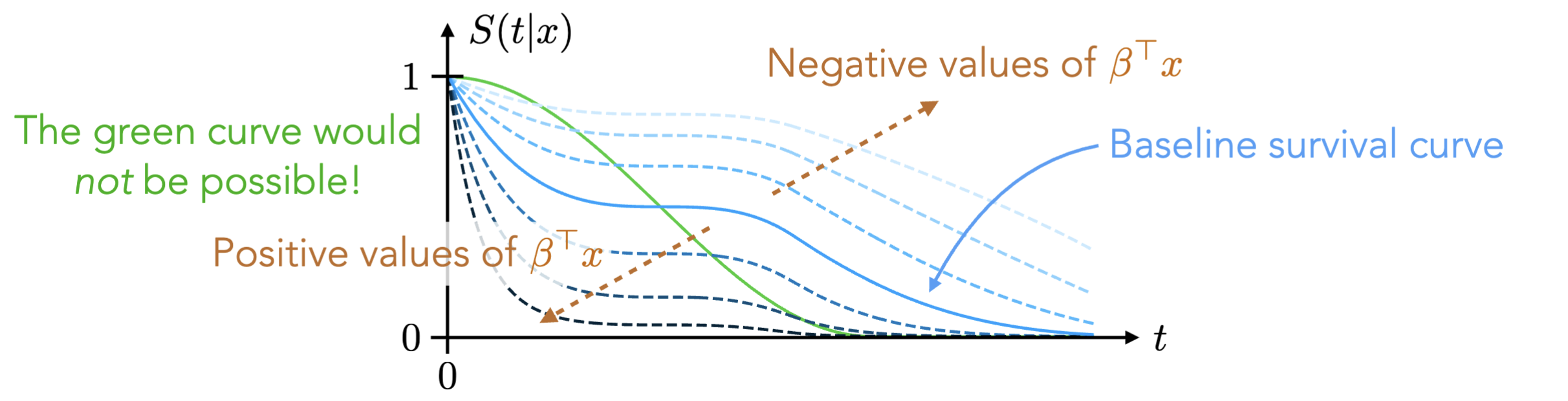
Under PH assumption, all survival curves must be powers of a baseline survival curve \(S_0(t)\)

Proportional hazard implications for the survival curve

Under PH assumption, survival curves must be powers of each other

• When \(\mathbf{x} \beta = 0\), we get the baseline survival curve

• When \(\mathbf{x} \beta > 0\) means shorter survival than the baseline

• When \(\mathbf{x} \beta < 0\) means longer survival than the baseline

From George Chen

Note that \(\mathbf{x} \beta = \beta^T \mathbf{x}\), where \(^T\) denotes transpose.

Testing proportional hazards

1. For categorical variables, we can check whether their \(\log(-\log(\text{survival functions}))\) are “parallel” (i.e., don’t cross, get closer or farther apart together over time)

2. For any variable, we can analyze the Schoenfeld residuals. For observation \(i\) that fails at \(t_i\) and feature \(k\):

\[ \text{Schoenfeld resid}_i = x_{ik} - \bar{x}_k(\beta, t_i) \]

where:

• \(x_{ik}\): \(k\)th feature for observation \(i\)

• \(t_i\): observed “death” or “failure” time for observation \(i\)

• \(\bar{x}_k(\beta, t_i)\): model-weighted average (or expected) value of the \(k\)th covariate among observations who are “at risk” right before \(t_i\)

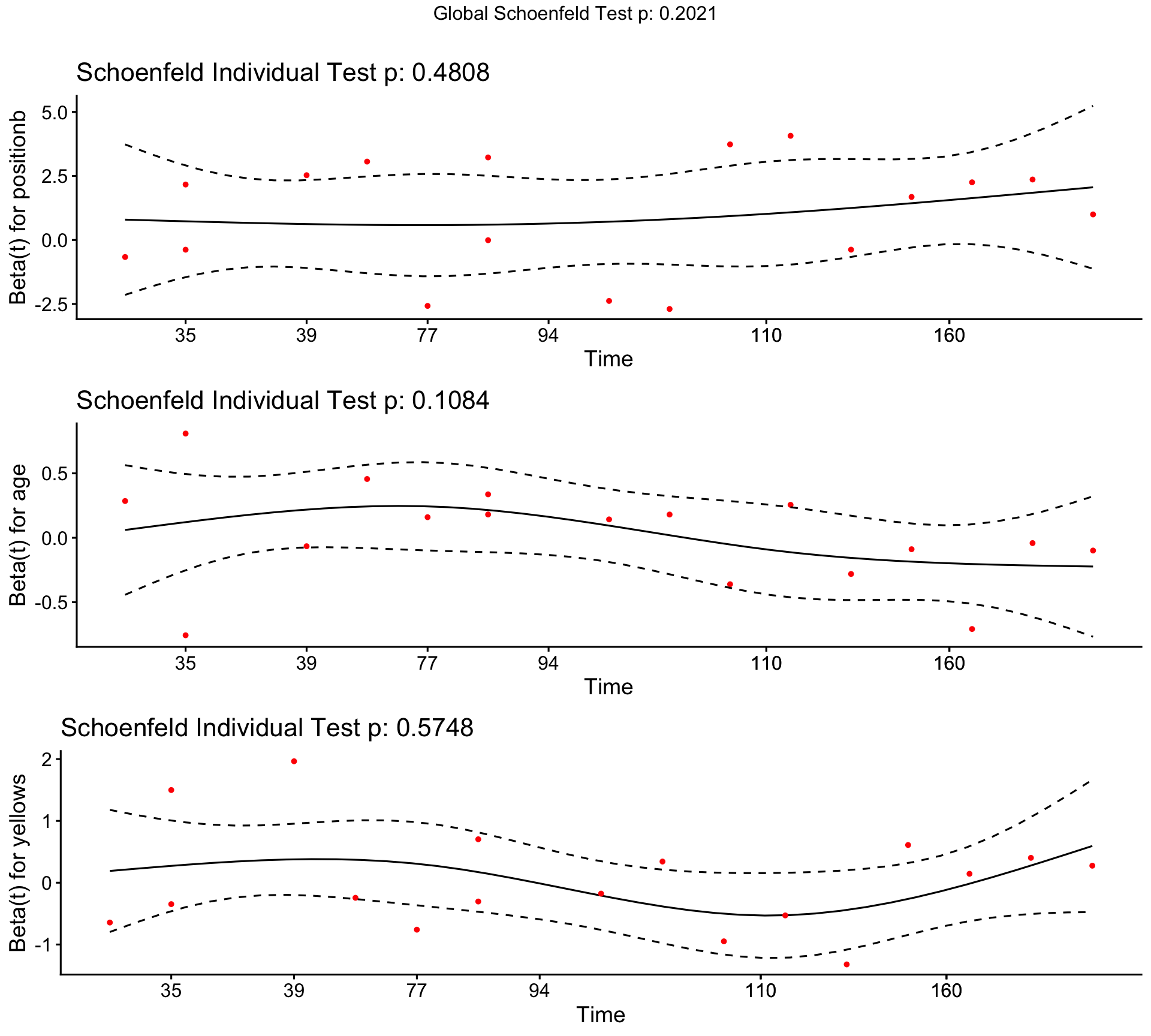
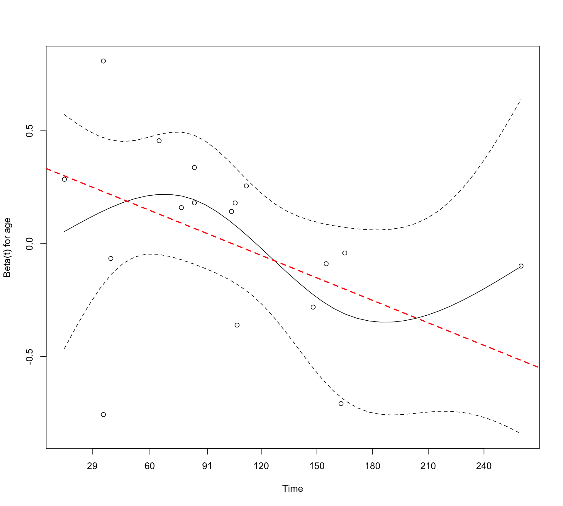
If PH assumption holds, Schoenfeld residuals should show no systematic trend over time

Interpreting coefficients

• We can calculate hazard ratio (HR) for any desired change in features, such as increasing a feature by one:

\[ \widehat{\text{HR}} = \frac{h(t \mid x_1 + 1, \dots, x_p)}{h(t \mid x_1, \dots, x_n)} = \frac{h_0(t) \exp(\beta_0 + \beta_1 (x_1 + 1) + \dots + \beta_p x_p)}{h_0(t) \exp(\beta_0 + \beta_1 x_1 + \dots + \beta_p x_p)} = \exp(\beta_1) \]

• Recall we can compute the 95% confidence interval for \(\beta_1\) as:

\[ \displaystyle [\hat{\beta}_1 - 1.96 \cdot \text{SE}(\hat{\beta}_1), \hat{\beta}_1 + 1.96 \cdot \text{SE}(\hat{\beta}_1)] \]

• So, the corresponding 95% confidence interval for \(\text{HR}\) is:

\[ \displaystyle [ \exp(\hat{\beta}_1 - 1.96 \cdot \text{SE}(\hat{\beta}_1)), \exp(\hat{\beta}_1 + 1.96 \cdot \text{SE}(\hat{\beta}_1))] \]

We can also perform hypothesis testing for \(\beta_1\) and HR using z-tests and drop-in-deviance tests, just like we did for GLMs!

Assessing calibration via concordance index

The Cox PH model ranks data points by their hazard

\[ \begin{aligned} \mathbf{x}_1 &\longrightarrow \mathbf{x}_1 \beta \\ \mathbf{x}_2 &\longrightarrow \mathbf{x}_2 \beta \\ &\cdots \\ \mathbf{x}_n &\longrightarrow \mathbf{x}_n \beta \end{aligned} \]

Example: if \(\mathbf{x}_1 \beta > \mathbf{x}_2 \beta\), then observation \(1\) has higher hazard than observation \(2\).

We compute the concordance index by:

1. Enumerating every pair of observations where at least one observation had a failure (i.e. exclude pairs where both observations are censored)

2. Computing the fraction of all such pairs where the unit with the earlier failure had a higher hazard

Measure of goodness-of-fit/predictive ability

Example in R

Data: Liverpool Football Club injuries

Injury data for Liverpool FC men’s first team (2017-2018 and 2018-2019 seasons), courtesy of the injurytools package

library(tidyverse)

injury_data <- read_csv("https://raw.githubusercontent.com/36-SURE/2026/main/data/liverpool_injury_data_17-19.csv") |>
  mutate(positionb = str_split_i(position, "_", 1)) |>
  filter(positionb != "Goalkeeper") 
#glimpse(injury_data)

Goal: estimate time until first injury for (non-Goalie) players given player-level attributes such as age and position

Data was web-scraped from https://www.transfermarkt.com/.

Fitting a Kaplan-Meier curve

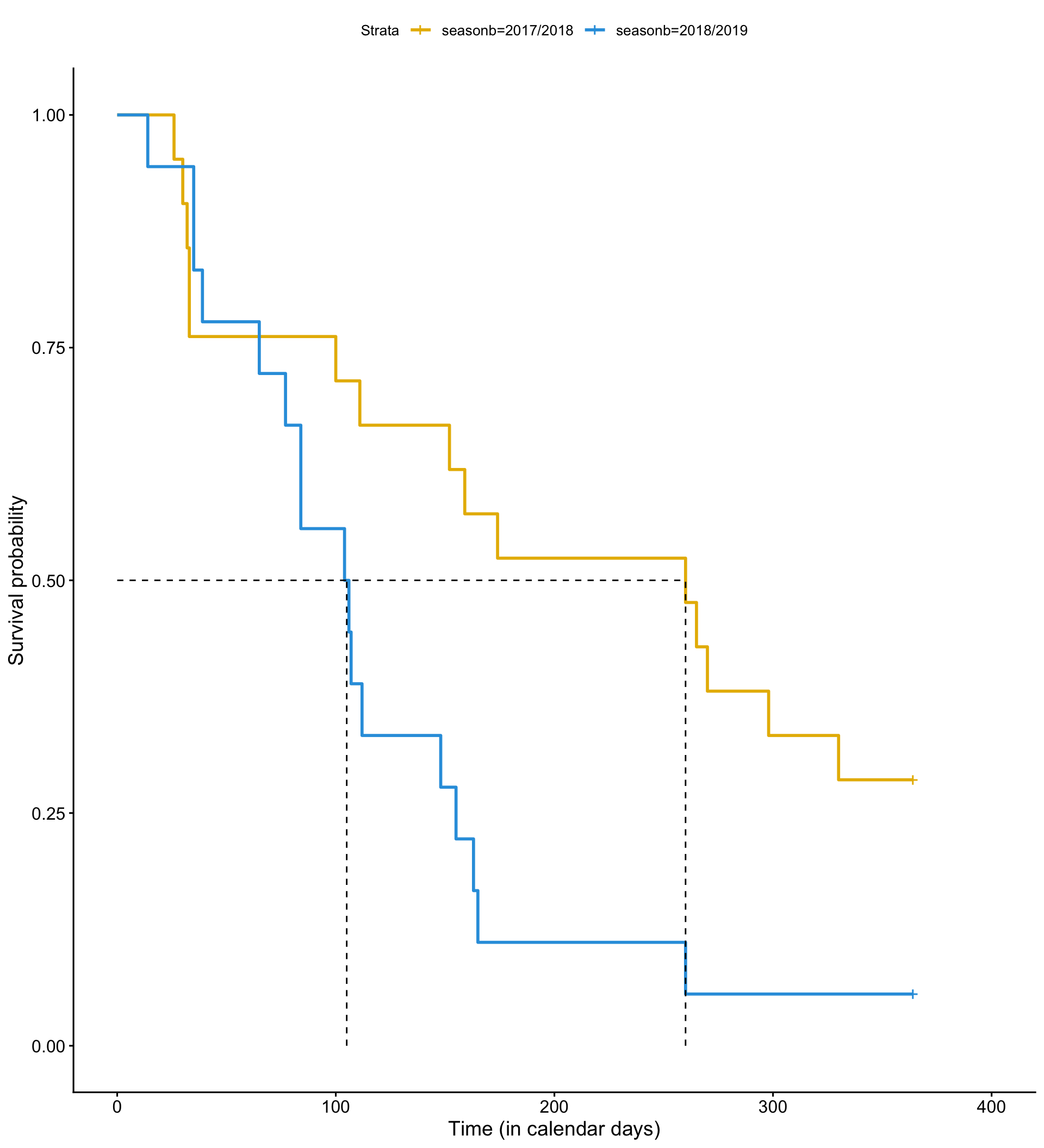
We can fitting the Kaplan-Meier curves using survfit() and Surv()

library(survival) # install.packages("survival")
km_fit <- survfit(Surv(tstop_day, status) ~ seasonb,
                  data = injury_data) 
km_fit

Call: survfit(formula = Surv(tstop_day, status) ~ seasonb, data = injury_data)

                   n events median 0.95LCL 0.95UCL
seasonb=2017/2018 21     15    260     111      NA
seasonb=2018/2019 18     17    105      77     163

Plotting the Kaplan-Meier curve using ggsurvplot()

library(survminer) # install.packages("survminer")
ggsurvplot(km_fit,  palette = c("#E7B800", "#2E9FDF"),
           surv.median.line = "hv",
           xlab = "Time (in calendar days)") 

Fitting the Cox PH model

We can fit Cox PH model with coxph() function:

library(gtsummary)
injury_data_sub <- injury_data |> filter(season == "18-19")

cfit <- coxph(Surv(tstop_day, status) ~ positionb + age + yellows,
              data = injury_data_sub)

tbl_regression(cfit, exponentiate = TRUE)

Characteristic	HR	95% CI	p-value
positionb
Attack	—	—
Defender	1.79	0.37, 8.71	0.5
Midfield	3.79	0.95, 15.1	0.059
age	1.02	0.84, 1.24	0.8
yellows	1.04	0.69, 1.56	0.9
Abbreviations: CI = Confidence Interval, HR = Hazard Ratio

Interpreting the Cox PH model

The estimated HR for Midfield is \(3.79\):

For Liverpool men’s FC first team players, midfielders were estimated to have 3.79 times the hazard of injury compared with attackers during 2018/2019 season, holding all other model variables constant (95% CI: [0.95, 15.1]).

The estimated HR for age is \(1.02\)

For Liverpool men’s FC first team players, a one-year increase in age was associated with 1.02 times increase in the hazard of injury, holding the other model variables constant (95% CI [0.84, 1.24]).

Schoenfeld residual diagnostics

cox.zph() tests whether the association of a given covariate \(X\) and the hazard is constant over time (i.e., whether PH assumption holds)

• \(H_0\) : The association between \(X\) and the hazard is constant over time

• \(H_1\): The association between \(X\) and the hazard is not constant (i.e., varies) over time

Given the global p-value is \(0.21\), we fail to reject that the association between our model covariates and the hazard is constant over time.

ggcoxzph(cox.zph(cfit))

Diagnosing non-PH via Kaplan-Meier curves

ggsurvplot(survfit(Surv(tstop_day, status) ~ positionb,
                   data = injury_data_sub), fun="cloglog",
           title = "Complementary Log-Log")

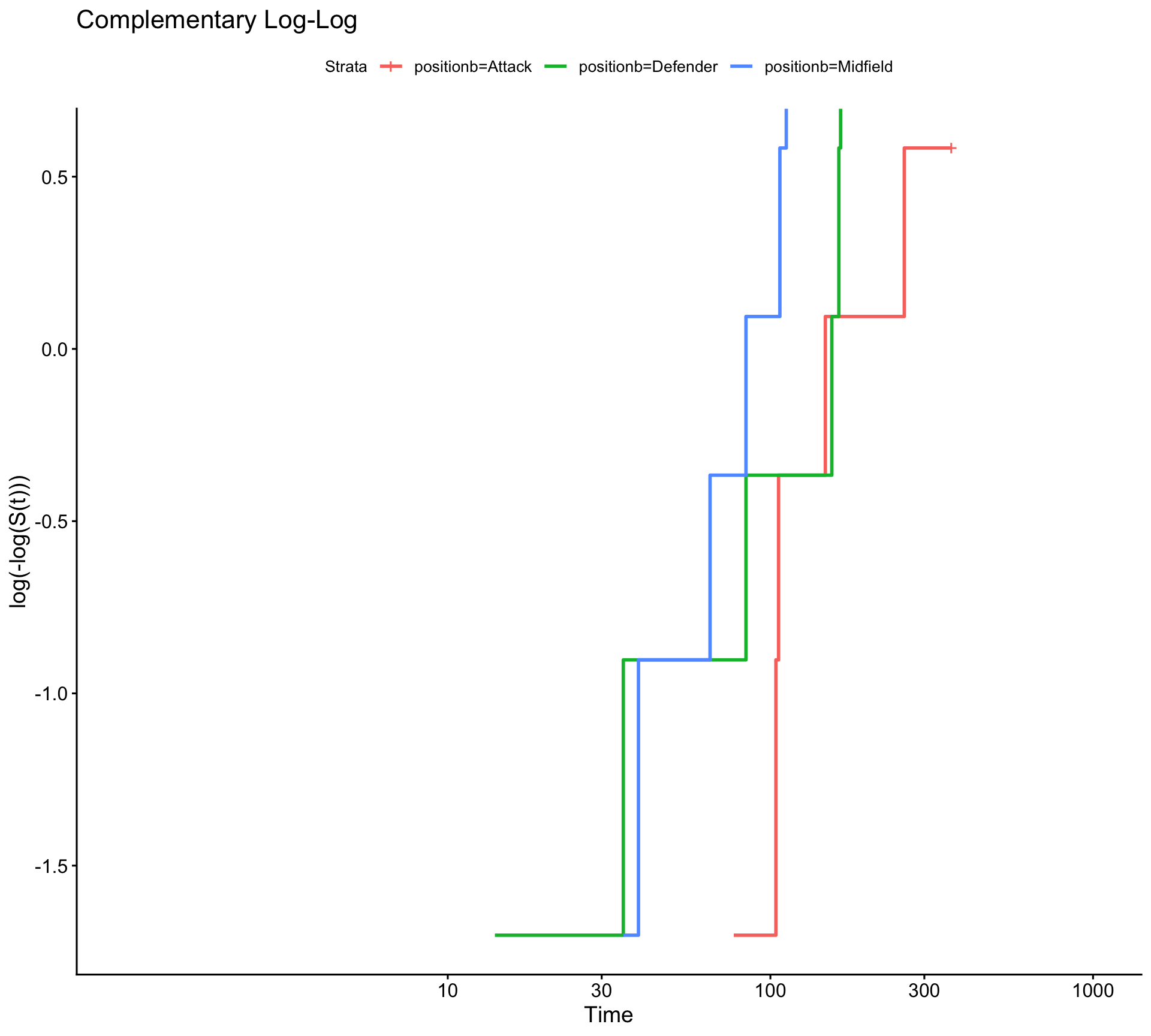
PH assumption for positionb definitely could be violated…(but it is hard to tell given how little data we have)

Handling non-proportional hazards

If the variable violating PH assumption is categorical:

• Stratify on the variable that violates PH (i.e., fit models separately)

• Fit Kaplan-Meier curves separately and perform a Wilcoxon test – note: this test is only valid if the survival curves don’t cross

If the variable violating PH assumption is continuous:

• Fit a model with a time dependent covariate. For example:

library(broom)
cfit_new <- coxph(Surv(tstop_day, status) ~ positionb + age + tt(age) + yellows,
                  data = injury_data_sub, tt = function(x, t, ...) x * t)
# tidy(cfit_new)

For more ideas, check out the paper, “Time-varying covariates and coefficients in Cox regression models”

Diagnosing (non-)linearity

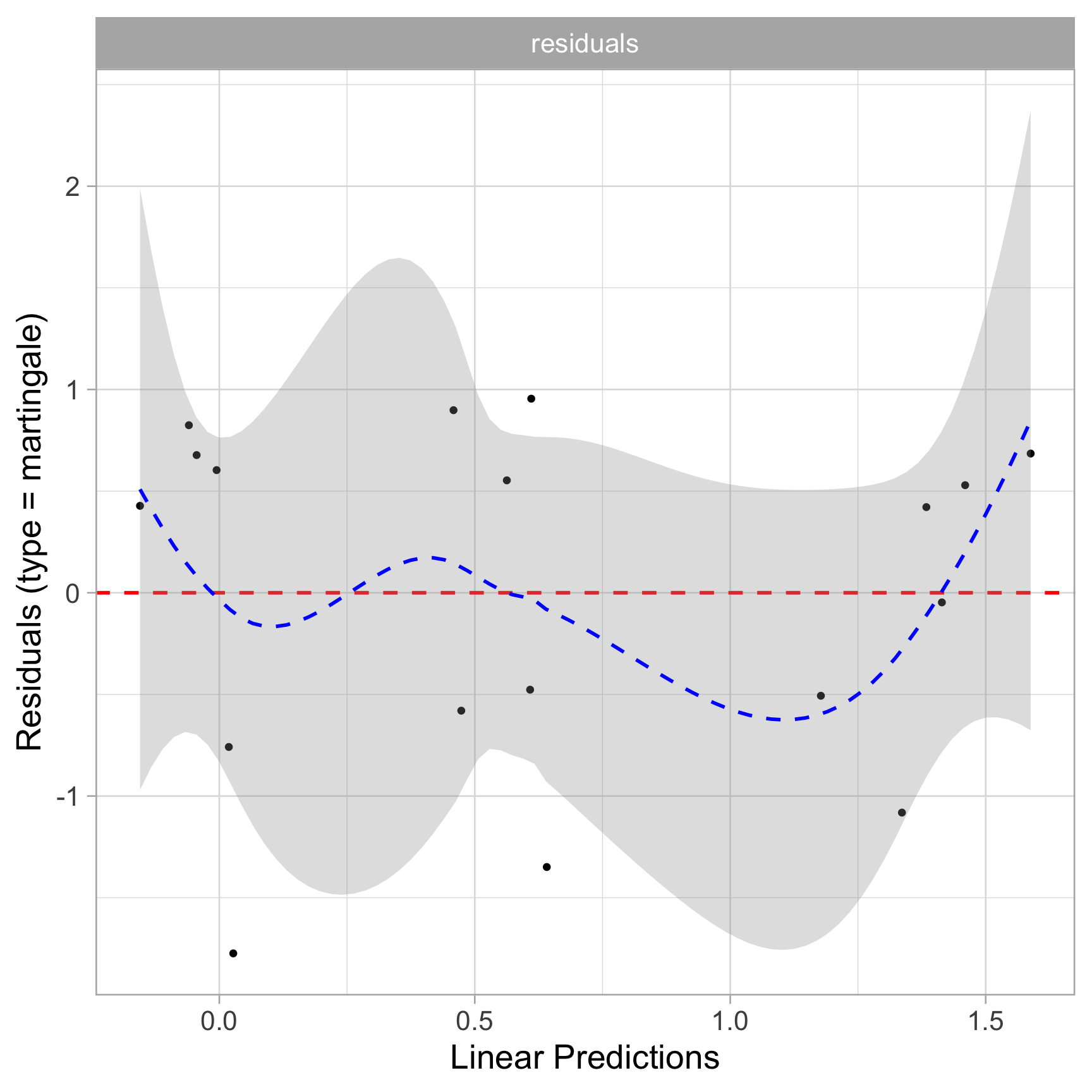
We can assess if the features are linearly related to the log hazard via martingale residuals.

For observation \(i\) with feature vector \(\mathbf{x}_i\):

\[ M_i = R_i - H(Y_i \mid \mathbf{x}_i) \]

where:

• \(Y_i\): \(\min\{T_i, C_i\}\)

• \(R_i\): indicator of whether the event occurred (aka if \(Y_i = T_i\))

• \(H(\cdot)\): cumulative hazard function

ggcoxdiagnostics(cfit, type = "martingale") + theme_light(base_size = 20)

Intuitive interpretation is that martingale residuals compare the number of observed events for each observation against the expected number under the model, given by \(H(\cdot)\) (technically, \(H(\cdot)\) is not a expected count, but close enough for our purposes).

Computing the concordance index

We can use concordance() or glance() to view the concordance index for our model

concordance(cfit) #glance(cfit), # could also compute on held-out data

Call:
concordance.coxph(object = cfit)

n= 18 
Concordance= 0.6291 se= 0.07191
concordant discordant     tied.x     tied.y    tied.xy 
        95         56          0          2          0 

Appendix

Visualizing time-dependent covariates

zph.tt <- cox.zph(cfit,  transform = function(t) t)
plot(zph.tt["age"])
abline(
  a = as.numeric(coef(cfit_new)["age"]),
  b = as.numeric(coef(cfit_new)["tt(age)"]),
  col = "red",
  lty = 2,
  lwd = 2
)

Proportional hazards with survival curves

With no features \(h_1(t) = h_0(t)e^\beta\). Hence, given the baseline survival curve \(\displaystyle S_0(t) = e^{-\int_0^t h_0(u) du}\):

\[ \begin{aligned} S_1(t) &= e^{-\int_0^t h_0(u)e^\beta du} \\ &= e^{-e^\beta \int_0^t h_0(u) du} \\ &= \left[e^{-\int_0^t h_0(u)du}\right]^{e^\beta} \\ \end{aligned} \]

Thus,

\[ \ln[-\ln(S_1(t))] = \beta + \ln[-\ln(S_0(t))] \]

Under PH, there is no “slope” just an intercept difference – hence the word “parallel”!

Proportional hazards with Schoenfeld residuals

We want \(\text{Pr}(i\text{th observation w/ }\mathbf{x}_i \text{ dies at }t_i \mid \text{at least one death at }t_i)\):

\[ \begin{aligned} &= \frac{\text{Pr}(i^{th} \text{ observation w/ } \mathbf{x}_i \text{ dies at } t_i)}{\text{Pr}(\text{at least one death at } t_i)} \\ &= \frac{\text{hazard at } t_i}{\text{sum over all patients at risk at time } t_i} \\ &= \frac{h_i(t_i)}{\sum_{j:t_j \geq t_i} h_j(t_i)} \\ &= \frac{e^{\mathbf{x}_i \beta }}{\sum_{j:t_j \geq t_i} e^{\mathbf{x}_j \beta}} \end{aligned} \]

We define:

\[ w_i(\beta, t_i) := \frac{e^{\mathbf{x}_i \beta }}{\sum_{j:t_j \geq t_i} e^{\mathbf{x}_j \beta}} \quad \text{and} \quad \bar{x}_k(\beta, t_i) := \sum_{j: t_j \geq t_i} x_{jk} w_i(\beta, t_i) \]

Related topics/extensions

• Accelerated failure time models (AFT models)

• Frailty models

• Deep survival models

Resources

• George Chen’s monograph on deep survival analysis models

• Alex Reinhart’s notes on survival analysis

• Jo Hardin’s notes on survival analysis

• Notes on Cox proportional hazards model estimation

Dataset preprocessing via injurytools

## 17/18
library(injurytools)
df_exposures1718 <- prepare_exp(df_exposures0 = 
                                  raw_df_exposures |> filter(season == "17/18"),
                                person_id     = "player_name",
                                date          = "year",
                                time_expo     = "minutes_played") |> 
  mutate(seasonb = date2season(date))
df_injuries1718 <- prepare_inj(df_injuries0   =
                                 raw_df_injuries |> filter(season == "17/18"),
                               person_id      = "player_name",
                               date_injured   = "from",
                               date_recovered = "until")
injd1718 <- prepare_all(data_exposures = df_exposures1718,
                        data_injuries  = df_injuries1718,
                        exp_unit = "matches_minutes")

injd1718 <- injd1718 |> 
  mutate(seasonb = date2season(tstart)) |> 
  ## join to have info such as position, age, citizenship etc.
  left_join(df_exposures1718, by = c("person_id" = "person_id", 
                                     "seasonb"   = "seasonb")) 

## create injd1718_sub:
##  - time to first injury
##  - equivalent tstart and tstop in calendar days
injd1718_sub <- injd1718 |> 
  mutate(tstop_day = as.numeric(difftime(tstop, tstart, units = "days"))) %>%
  group_by(person_id) |>  ## important
  mutate(tstop_day = cumsum(tstop_day),
         tstart_day = lag(tstop_day, default = 0)) |> 
  ungroup() |> 
  dplyr::select(person_id:tstop_minPlay, tstart_day, tstop_day, everything()) |> 
  filter(enum == 1) ## time to first injury

## 18/19
df_exposures1819 <- prepare_exp(df_exposures0 = 
                                  raw_df_exposures |> filter(season == "18/19"),
                                person_id     = "player_name",
                                date          = "year",
                                time_expo     = "minutes_played") |> 
  mutate(seasonb = date2season(date))
df_injuries1819 <- prepare_inj(df_injuries0   = 
                                 raw_df_injuries |> filter(season == "18/19"),
                               person_id      = "player_name",
                               date_injured   = "from",
                               date_recovered = "until")
injd1819 <- prepare_all(data_exposures = df_exposures1819,
                        data_injuries  = df_injuries1819,
                        exp_unit = "matches_minutes")

injd1819 <- injd1819 |> 
  mutate(seasonb = date2season(tstart)) |> 
  ## join to have info such as position, age, citizenship etc.
  left_join(df_exposures1819, by = c("person_id" = "person_id", 
                                     "seasonb"   = "seasonb")) 

## create injd1819_sub:
##  - time to first injury
##  - equivalent tstart and tstop in calendar days
injd1819_sub <- injd1819 |> 
  mutate(tstop_day = as.numeric(difftime(tstop, tstart, units = "days"))) %>%
  group_by(person_id) |>  ## important
  mutate(tstop_day = cumsum(tstop_day),
         tstart_day = lag(tstop_day, default = 0)) |> 
  ungroup() |> 
  dplyr::select(person_id:tstop_minPlay, tstart_day, tstop_day, everything()) |> 
  filter(enum == 1) ## time to first injury

injd_sub <- bind_rows("17-18" = injd1718_sub,
                      "18-19" = injd1819_sub,
                      .id = "season")