Advanced topics: SQL

CMSACamp 2026

Department of Statistics & Data Science
Carnegie Mellon University

Background

Recall: data science workflow

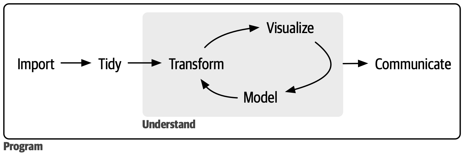
So far, we have primarily focused on tidy, understand, and communicate steps, taking the import step for granted

In industry, most data live in SQL databases and are too big to live in our laptops

Therefore: being able to (efficiently) extract data from SQL databases is vital for success

Why aren’t R/Python alone sufficient for this purpose?

SQL databases allow you to persistently store and organize data

Can handle large volumes of data and easily scalable

Support a streamlined Extract-Transform-Load (ETL) process for streaming data

Provide access management restrictions to specific data, e.g., health records

Allow for explicit linkages across tables (primary and foreign keys)

Enable indexes to be defined on tables for efficiency, e.g., date/time fields

Typical workflow: use R for accessing subsets of data from a SQL database for modeling

What is a database?

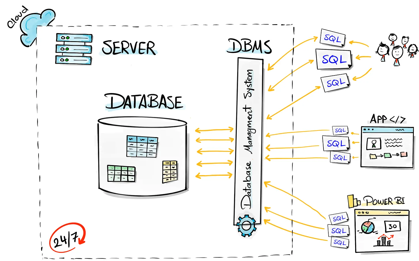
A database is an organized collection of data that is managed by a database management system (DBMS)

A DBMS is the software with which users interact to obtain or analyze data stored in a database
Contrast to a file-based system that manage and organize data as individual files on storage

Advantages of DBMSs include:

Control of data redundancy
Ensure data consistency across users
Improved security and control over data-sharing
Improved data integrity
Economy of scale

BUT…DBMSs also can be more complex, costly, and have a higher impact of failure

Intro to SQL (Structured Query Language)

SQL provides a consistent grammar (Structured Language) for asking and answering questions (Queries) about collected data
Allows us to communicate with data stored in a database via a (relational) DBMS

SQL dialects

SQL has multiple dialects, such as:

MySQL
SQLite (what we use today)
DuckDB
PostgreSQL
Google BigQuery
Microsoft Access SQL

Multiple dialects allow SQL to be tailored to the specific needs and capabilities of different DBMSs

Different SQL dialects are quite similar to each other

So, while we use SQLite today, you will be able to quickly pickup whichever dialect your institution/employer uses

SQL tables are nouns, on which you ask targeted queries

SQL tables are just 2D representations of data

A collection of columns (variables) and observations

These are similar to data frames/tibbles in R
- You’ve already worked with them in R - yay!

year	month	day	dep_time	sched_dep_time	dep_delay	arr_time	sched_arr_time	arr_delay	carrier	flight	tailnum	origin	dest	air_time	distance	hour	minute	time_hour
2013	1	1	517	515	2	830	819	11	UA	1545	N14228	EWR	IAH	227	1400	5	15	2013-01-01 05:00:00
2013	1	1	533	529	4	850	830	20	UA	1714	N24211	LGA	IAH	227	1416	5	29	2013-01-01 05:00:00
2013	1	1	542	540	2	923	850	33	AA	1141	N619AA	JFK	MIA	160	1089	5	40	2013-01-01 05:00:00

SQL grammar has built-in keywords (verbs)

SQL keywords are verbs which allow you to systematically query tables

Example: starting with flights data from nycflights13 package

Each row represents a flight departed from NYC in 2013
336,000+ observations and 19 columns (variables)

SQL code

SELECT dest, month,
  MIN(arr_delay) AS mnd,
  MAX(arr_delay) AS mxd,
  AVG(arr_delay) AS avd
FROM flights
GROUP BY dest, month
ORDER BY dest, month DESC
LIMIT 6;

We will go through what each of these functions does during this presentation!

dest	month	mnd	mxd	avd
ABQ	12	-38	149	30.3225806
ABQ	11	-61	34	-8.0333333
ABQ	10	-35	138	0.2903226
ABQ	9	-43	109	-0.3666667
ABQ	8	-55	98	-3.5483871
ABQ	7	-45	153	17.0967742

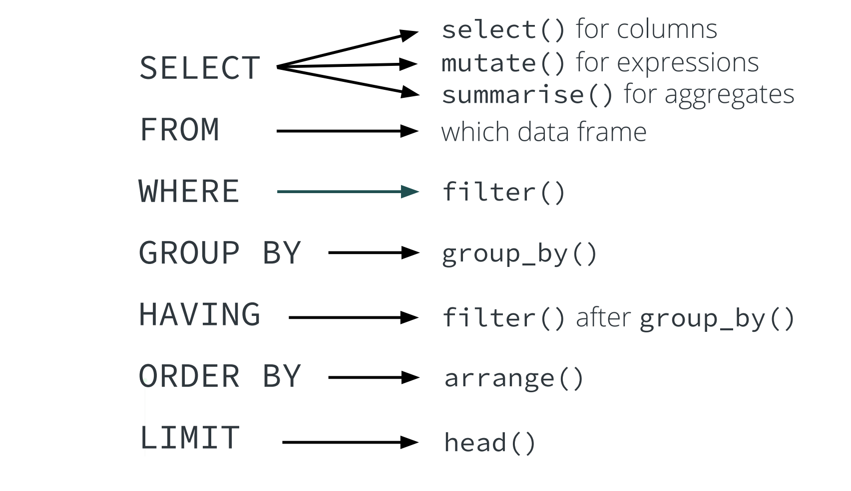
SQL keywords map onto `dplyr` verbs

Today: `nycflights13` database

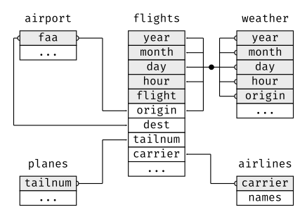
Contains flight info for NYC departures to various US destinations in 2013

flights: all NYC departures in 2013
weather: hourly data for each airport
planes: construction info for each plane
airports: airport names and locations
airlines: two letter carrier codes/names

Establishing a SQL connection within `R`

We use SQLite: “small, fast, self-contained, high-reliability, full-featured, SQL database engine”

#install.packages(c("DBI", "dittodb", "RSQLite", "nycflights13")) need to install all these
library(DBI)
library(dittodb)
library(RSQLite)

# establishing connection via sqlite
# ":memory:" is a special path that creates an in-memory database
# other database drivers require more details (like user, password, host, port, etc.)
con_air <- DBI::dbConnect(RSQLite::SQLite(), ":memory:") 
# creates a database including a few tables from the nycflights13 dataset with con_air connection
dittodb::nycflights13_create_sql(con_air)

The function dbListTables() tells us what tables exist in the airlines database

DBI::dbListTables(con_air)

[1] "airlines" "airports" "flights"  "planes"   "weather"

SQL tables as a `tibble`

A tbl is different than a tibble

tbl is a pointer to a remote object
tibble is a dataframe in your local environment

flights_tbl <- tbl(con_air, "flights")
dim(flights_tbl)  #head(flights_tbl, n = 3)

[1] NA 19

We can use dplyr syntax on tbl objects

dist_sum <- flights_tbl |>
  summarize(min_year = min(distance), max_year = max(distance))

Since flights_tbl is a tbl, the work done above was done in SQL:

show_query(dist_sum)

<SQL>
SELECT MIN(`distance`) AS `min_year`, MAX(`distance`) AS `max_year`
FROM `flights`

SQL tables as a `tibble`

collect() copies a SQL table from its remote server location to the local memory location in R

flights_tibble <- flights_tbl |> dplyr::collect()

# dim(flights_tibble)
head(flights_tibble, n = 3)

# A tibble: 3 × 19
   year month   day dep_time sched_dep_time dep_delay arr_time sched_arr_time
  <int> <int> <int>    <int>          <int>     <dbl>    <int>          <int>
1  2013     1     1      517            515         2      830            819
2  2013     1     1      533            529         4      850            830
3  2013     1     1      542            540         2      923            850
# ℹ 11 more variables: arr_delay <dbl>, carrier <chr>, flight <int>,
#   tailnum <chr>, origin <chr>, dest <chr>, air_time <dbl>, distance <dbl>,
#   hour <dbl>, minute <dbl>, time_hour <dbl>

A tibble (locally in R) takes up much more memory than a tbl (pointing to remote object in SQL)

flights_tbl |>
  object.size() |>
  print(units = "Kb")

6.4 Kb

flights_tibble |>
  object.size() |>
  print(units = "Kb")

39696.8 Kb

Different ways to query in Quarto

Using the dbplyr R package (loaded with tidyverse) will directly translate dplyr code into SQL

flights_tbl |>
  summarize(min_year = min(distance), max_year = max(distance)) # what we previously did

Using the DBI R package, we can send SQL queries through an r chunk

DBI::dbGetQuery(con_air,
                "SELECT MIN(distance) AS min_year,
                MAX(distance) AS max_year
                FROM flights")

Using a sql chunk, we can write actual SQL code inside a Quarto document

SELECT MIN(distance) AS min_year,
       MAX(distance) AS max_year
FROM flights

We will primarily use the third option today

SQL queries ordering

Queries in SQL start with SELECT keyword and consist of several keywords which must be written in the following order:

SELECT
FROM
JOIN
WHERE
GROUP BY
HAVING
ORDER BY
LIMIT

A semicolon (;) is typically used to indicate the termination of a SQL statement

`SELECT` to subset columns from a table

Syntax: SELECT <column_name> FROM <table_name>

Let’s look at 10 rows and all variables from the flights table:

SELECT * FROM flights LIMIT 10;

Notes:

It’s best practice to always use LIMIT when just selecting columns from a table
The asterisk (*) means return all (any) columns
SQL will return any 10 rows, so the original flights order may not be preserved

`SELECT` to subset columns from a table

Let’s look at 10 rows and only the dep_time, arr_time, and flight variables from the flights table:

SELECT dep_time, arr_time, flight FROM flights LIMIT 10;

The equivalent dplyr code is:

flights |> select(dep_time, arr_time) |> head(10)

Notes:

The original flights ordering is preserved in dplyr
SQL operates on sets of observations, which are an unordered collection
We’ll later control ordering explicitly in SQL using ORDER BY

`SELECT` to create new variables

Suppose we want to measure of average speed (in miles per hour) for each flight:

SELECT flight, distance/(air_time/60) AS speed FROM flights LIMIT 10;

AS speed says that we want to name our new column speed, instead of distance/(air_time/60)

In dplyr, we have the mutate() verb

flights |> 
  mutate(speed = distance/(air_time/60)) |>
  select(flight, speed) |>
  head(10)

Takeaway: SELECT in SQL serves to pick existing columns or to create new ones

We can also aggregate on columns via `SELECT`

SQL has built in aggregate functions: MIN, MAX, COUNT, SUM, AVG, … (some depend on specific SQL dialect, like MEDIAN)

Let’s get the minimum and maximum air time for the flights in our SQL table (luckily air_time is in minutes not hours…)

SELECT MIN(air_time) AS min_ar, MAX(air_time) AS max_ar FROM flights;

Like dplyr, SQL also has a COUNT function. We can use it to get the total number of observations in our table

SELECT COUNT(*) AS num_obs FROM flights;

Filtering observations `WHERE` a criteria is met

Suppose we want to filter to only observations that originated from JFK airport and limit our results to ten rows (keeping all columns):

SELECT * FROM flights WHERE origin = "JFK" LIMIT 10;

Note: SQL uses = NOT ==

Like in base R, we can use ! to negate the equal sign statement

SELECT * FROM flights WHERE origin != "JFK" LIMIT 10;

SQL supports other logical operators, such as: <, <=, >, >=

`WHERE` to find value IN or NOT IN a range?

Find 20 records which have a tail number matching either “N593JB” or “N532UA”:

SELECT * FROM flights WHERE tailnum IN ("N593JB", "N532UA") LIMIT 20;

Find 10 records which are:

From neither December nor January
Have an arrival delay greater than 120 minutes

SELECT * FROM flights WHERE month NOT IN (1, 12) AND arr_delay > 120 LIMIT 10;

Missing values in SQL

NULL refers to missing values in SQL

We have a substantial number of observations that are missing wind_gust variable:

SELECT COUNT(*) AS num_obs FROM weather WHERE wind_gust IS NULL;

We can remove the missing values using wind_gust is NOT NULL

SELECT * FROM weather WHERE wind_gust IS NOT NULL LIMIT 20;

Note: wind_gust != NULL does not work as NULL values don’t match this way in SQL

This is different from base R and dplyr

`GROUP BY` variables and do aggregate calculations

Let’s get the minimum, maximum, and average arrival delay by month, day, and destination:

SELECT dest, month, day,
       MIN(arr_delay) AS mnd,
       MAX(arr_delay) AS mxd,
       AVG(arr_delay) AS avd
FROM flights
GROUP BY dest, month, day
LIMIT 10;

Filtering aggregated values with `HAVING`

Given number of plane engines, how many had less than 200 manufacturers?

SELECT engines, COUNT(*) AS tot_num
 FROM planes
 GROUP BY engines
 HAVING tot_num < 200;

`ORDER BY` columns when displaying output

Get minimum, maximum, and average arrival delay by month day and destination:

SELECT dest, month, day,
       MIN(arr_delay) AS mnd, MAX(arr_delay) AS mxd,
       AVG(arr_delay) AS avd
FROM flights
GROUP BY dest, month, day
ORDER BY dest, month DESC, day
LIMIT 10;

Like dplyr, the ordering in SQL is ascending by default, unless you specify descending with DESC

Try it yourself: which destination had the longest average delays?

Spot the syntax mistakes

FROM flights
GROUP BY dest
SELECT AVG(arr_delay) AS avd
ORDER BY DESC avd;

Other handy SQL functions

DISTINCT can be used to obtain only the unique values (or combinations) from a table.

Getting the first ten records of unique carrier and flight number combinations, ordered by carrier and then flight number:

SELECT DISTINCT carrier, flight FROM flights ORDER BY carrier, flight LIMIT 10;

We also can use CASE WHEN in SQL (analogous to case_when() in dplyr)

Creating a new factor variable called delay_type:

SELECT year, month, day, arr_delay,
       CASE WHEN arr_delay < 0 THEN "Early"
       WHEN arr_delay = 0 THEN "On Time"
       WHEN arr_delay > 0 THEN "Late"
       ELSE "Unknown"
  END AS delay_type
FROM flights LIMIT 10;

Subqueries in SQL

Subqueries are queries that are nested inside another SQL query
Help us get more automation over filtering

Suppose we want to count total flights with destination codes starting with “M”, grouped by code

We could first get all destination codes starting with “M” (LIKE "M%" does wildcard matching)

SELECT DISTINCT dest FROM flights WHERE dest LIKE "M%"

Then, we could manually type out this list in are query but this is tedious are prone to error

SELECT dest, COUNT(*) as tot_flights
 FROM flights
 WHERE dest IN ("MIA", "MCO", "MSP", "MSY", "MKE", "MEM", "MYR", "MDW",
 "MHT", "MSN", "MCI", "MTJ", "MVY")
 GROUP BY dest

Additional worry: what if a new destination code is added that starts with “M”?

Subqueries in SQL

SELECT dest, COUNT(*) as tot_flights
 FROM flights
 WHERE dest IN (SELECT DISTINCT dest FROM flights WHERE dest LIKE "M%")
 GROUP BY dest

Takeaway: subqueries result in more automated, scalable, and expressive code

Relating information between tables in SQL

How to get the count of total flights in Jun/Jul by plane carrier name?

SELECT carrier, COUNT(*) as tot_flights
 FROM flights
 WHERE month IN (6, 7)
 GROUP BY carrier

Almost there…but we want the carrier name, not carrier code

How can we modify our query to obtain and use this carrier name information?

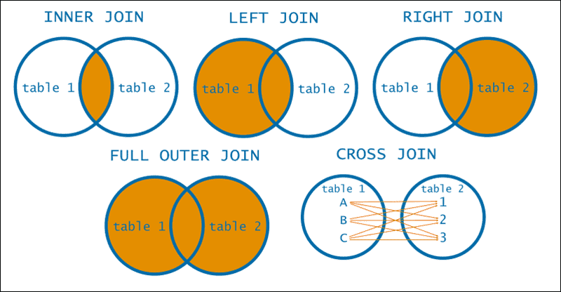
We can use joins!

Joining in SQL

Recall that SQL is a query language that works on relational databases
The syntax for tying together information from multiple tables is done with a JOIN clause

A JOIN clause requires four pieces of information:

The name of the first table you want to JOIN
The type of JOIN being used
The name of the second table you want to JOIN
The condition(s) under which the records in the first table should match records in the second table

Venn diagrams describing different JOINs, image credit: phoenixNAP

Interlude: keys in SQL

Keys are useful for the following:

Creating relationships between two tables
Keeping data consistent and valid in the database
Helping in fast retrieval of data
Maintaining uniqueness in a table

Primary key: constraint that uniquely identifies each record in a table (e.g., studentID)
- Must be unique and not null
- Only one allowed per table
Foreign key: constraint that establishes a link between two tables
- Refers to the primary key in another table

These are extremely useful for joining/relating two tables in a SQL database!

Joining in SQL

airlines: carrier code is a PRIMARY KEY since it uniquely identifies each observation
flights carrier code is a FOREIGN KEY that corresponds to the carrier code PRIMARY KEY in airlines — it is not a unique identifier of observations in flights

We can use the idea of a LEFT JOIN to link the keys:

SELECT al.name AS airline, COUNT(*) as tot_flights
FROM flights AS fl
LEFT JOIN airlines AS al
  ON al.carrier = fl.carrier
WHERE month IN (6, 7)
GROUP BY al.name

Note: we use table aliases (e.g., “al” for “airlines”) to avoid reference ambiguities

This gives us the airline names based on the carrier code column!

Saving SQL query outputs as R objects

We can use --|output.var: "name_of_variable" inside the {sql} chunk to save query output to the R environment

SELECT al.name AS airline, COUNT(*) as tot_flights
FROM flights AS fl
LEFT JOIN airlines AS al
  ON al.carrier = fl.carrier
WHERE month IN (6, 7)
GROUP BY al.name

This allows us to use query output for further analysis or visualizations in R

head(tot_airline_flights, n = 3)

                      airline tot_flights
1 AirTran Airways Corporation         515
2        Alaska Airlines Inc.         122
3      American Airlines Inc.        5639

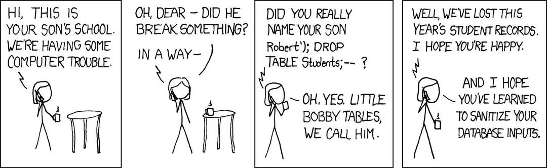
Destructive actions in SQL

In SQL, you can run commands that alter database schemas or permanently erase and modify data without automatically generating backups.

These are called destructive actions. Examples include:

DROP: deletes entire database objects (like tables, views, indexes, or the entire database) along with their data and structural definitions
TRUNCATE: instantly removes all rows from a table, resetting the table to its initial empty state
DELETE: removes rows from a table
UPDATE: modifies existing data in the database

Running DELETE (or UPDATE) without a WHERE clause will delete (or overwrite) every single row in the table

SQL best practices

Before running any destructive action, you should:

Verify the statement with SELECT
Use a SQL transaction block for testing

Terminate the SQL connection when finished

DBI::dbDisconnect(con_air, shutdown = TRUE)

Protecting your username and password

In practice, we will often have to put in credentials to connect to a SQL database

con_air <- DBI::dbConnect(
  RSQLite::SQLite(),
  dbname = "airlines",
  host = ???,
  user = ???,
  password = ???
)

So, how do we do this without leaking our username/password?

Edit the .Renviron file

# For a specific project (recommended)
usethis::edit_r_environ(scope = "project")

Then use Sys.getenv() to safely pull the variables into our SQL connection wrapper without sharing our username or password

Sys.getenv("SQL_PASSWORD")

[1] "scotty_dawg_47"

Appendix

SQL command typology

You may hear SQL commands split into subsets by their purpose:

Data Definition Language (DDL): commands to create and define the structure of a database
- CREATE, ALTER, DROP
Data Manipulation Language (DML): commands to handle data within tables
- INSERT, UPDATE, DELETE
Data Query Language (DQL): commands to retrieve or query data from tables
- SELECT, WHERE, LIMIT

Resources

List of resources consulted for building these slides:

Advanced topics: SQL

Background

Recall: data science workflow

Why aren’t R/Python alone sufficient for this purpose?

What is a database?

Intro to SQL (Structured Query Language)

SQL dialects

SQL tables are nouns, on which you ask targeted queries

SQL grammar has built-in keywords (verbs)

SQL keywords map onto dplyr verbs

Today: nycflights13 database

Establishing a SQL connection within R

SQL tables as a tibble

SQL tables as a tibble

Different ways to query in Quarto

SQL queries ordering

SELECT to subset columns from a table

SELECT to subset columns from a table

SELECT to create new variables

We can also aggregate on columns via SELECT

Filtering observations WHERE a criteria is met

WHERE to find value IN or NOT IN a range?

Missing values in SQL

GROUP BY variables and do aggregate calculations

Filtering aggregated values with HAVING

ORDER BY columns when displaying output

Spot the syntax mistakes

Other handy SQL functions

Subqueries in SQL

Subqueries in SQL

Relating information between tables in SQL

Joining in SQL

Interlude: keys in SQL

Joining in SQL

Saving SQL query outputs as R objects

Destructive actions in SQL

SQL best practices

Protecting your username and password

Appendix

SQL command typology

Resources

SQL keywords map onto `dplyr` verbs

Today: `nycflights13` database

Establishing a SQL connection within `R`

SQL tables as a `tibble`

SQL tables as a `tibble`

`SELECT` to subset columns from a table

`SELECT` to subset columns from a table

`SELECT` to create new variables

We can also aggregate on columns via `SELECT`

Filtering observations `WHERE` a criteria is met

`WHERE` to find value IN or NOT IN a range?

`GROUP BY` variables and do aggregate calculations

Filtering aggregated values with `HAVING`

`ORDER BY` columns when displaying output