Supervised learning: logistic regression

SURE 2024

Department of Statistics & Data Science
Carnegie Mellon University

Background

Classification

Categorical variables take values in an unordered set with different categories
Classification: predicting a categorical response \(Y\) for an observation (since it involves assigning the observation to a category/class)
Often, we are more interested in estimating the probability for each category of the response \(Y\)
Classification is different from clustering, since we know the true label \(Y\)
We will focus on binary categorical response (categorical response variables with only two categories)
- Examples: whether it will rain or not tomorrow, whether the kicker makes or misses a field goal attempt

Logistic regression

Review: in linear regression, the response variable \(Y\) is continuous
Logistic regression is used to model binary outcomes (i.e. \(Y \in \{0, 1\}\))
Similar concepts from linear regression
- tests for coefficients
- indicator variables
- model selection techniques
- regularization
Other concepts are different
- interpretation of coefficients
- residuals are not normally distributed
- model evaluation

Why not linear regression for categorical data?

From ISLR:

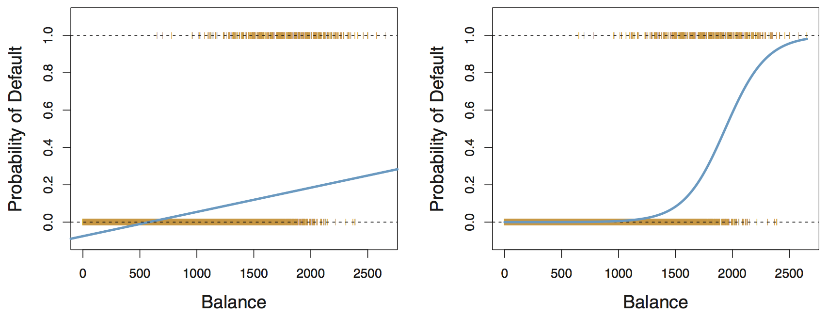
Linear regression

predicted probabilities might be outside the \([0, 1]\) interval

Logistic regression

all probabilities lie between 0 and 1

Logistic regression

Logistic regression models the probability of success \(p(x)\) of a binary response variable \(Y \in \{0, 1\}\)
To limit the regression between \([0, 1]\), we use the logit function, or the log-odds ratio

\[ \log \left( \frac{p(x)}{1 - p(x)} \right) = \beta_0 + \beta_1 x_1 + \cdots + \beta_p x_p \]

or equivalently,

\[ p(x) = \frac{e^{\beta_0 + \beta_1 x_1 + \cdots + \beta_p x_p}}{1 + e^{\beta_0 + \beta_1 x_1 + \cdots + \beta_p x_p}} \]

Note: \(p(x)= P(Y = 1 \mid X = x) = \mathbb E[Y \mid X = x]\)

Maximum likelihood estimation (MLE)

Likelihood function: how likely to observe data for given parameter values \[L(\theta) = \prod_{i=1}^n f(y_i; \theta)\]

Goal: find values for parameters that maximize likelihood function (i.e., MLEs)

Why: likelihood methods can handle variety of data types and assumptions

How: typically numerical approaches and optimization techniques
- Easier to work with log-likelihood (sums compared to products)

Example: linear regression MLE

Reminder: probability density function (pdf) for a normal distribution \[f(y \mid \mu, \sigma) = \frac{1}{\sqrt{2\pi \sigma^2}} e^{\frac{-(y - \mu) ^ 2}{2 \sigma^2}}\]

Consider a simple linear regression model (with an intercept and one predictor) \[y_i = \beta_0 + \beta_1 x_i + \epsilon_i, \quad \epsilon_i \sim N(0, \sigma^2)\]

Then \(\qquad \displaystyle L(\beta_0, \beta_1, \sigma) = \prod_{i=1}^n f(y_i \mid x_i; \beta_0, \beta_1, \sigma) = \prod_{i=1}^n \frac{1}{\sqrt{2\pi \sigma^2}} e^{\frac{-(y_i - \beta_0 - \beta_1 x_i) ^ 2}{2 \sigma^2}}\)

And \(\qquad \displaystyle \log L(\beta_0, \beta_1, \sigma) = -\frac{n}{2} \log 2\pi - \frac{n}{2} \log \sigma^2 - \frac{1}{2 \sigma^2} \sum_{i=1}^n (y_i - \beta_0 - \beta_1x_1)^2\)

We can then use calculus to find the optimal parameter values. For more details, see here

Major difference between linear and logistic regression

Logistic regression involves numerical optimization

\(y_i\) is observed response for \(n\) observations, either 0 or 1

We need to use an iterative algorithm to find \(\beta\)’s that maximize the likelihood \[\prod_{i=1}^{n} p\left(x_{i}\right)^{y_{i}}\left(1-p\left(x_{i}\right)\right)^{1-y_{i}}\]

Newton’s method: start with initial guess, calculate gradient of log-likelihood, add amount proportional to the gradient to parameters, moving up log-likelihood surface

This means logistic regression runs more slowly than linear regression

if you’re interested: iteratively re-weighted least squares, see here

Inference with logistic regression

Major motivation for logistic regression (and all GLMs) is inference
- How does the response change when we change a predictor by one unit?

For linear regression, the answer is straightforward

\[\mathbb{E}[Y \mid x] = \beta_0 + \beta_1 x_1 + + \cdots + \beta_p x_p\]

For logistic regression, it is a little less straightforward

\[\mathbb E[Y \mid x] = \frac{e^{\beta_0 + \beta_1 x_1 + \cdots + \beta_p x_p}}{1 + e^{\beta_0 + \beta_1 x_1 + \cdots + \beta_p x_p}}\]

Note:

The predicted response varies non-linearly with the predictor variable values
Interpretation on the odds scale

The odds interpretation

The odds of an event are the probability of the event divided by the probability of the event not occurring

\(\displaystyle \text{odds} = \frac{\text{probability}}{1 - \text{probability}}\)
\(\displaystyle \text{probability} = \frac{\text{odds}}{1 + \text{odds}}\)

Example: Rolling a fair six-sided die

The probability of rolling a 2 is 1/6
The odds of rolling a 2 is 1 to 5 (or 1:5)

The odds interpretation

Suppose we fit a simple logistic regression model (with one predictor), and say the predicted probability is 0.8 for a particular predictor value

This means that if we were to repeatedly sample response values given that predictor variable value: we expect class 1 to appear 4 times as often as class 0 \[\text{odds} = \frac{\mathbb{E}[Y \mid x]}{1-\mathbb{E}[Y \mid x]} = \frac{0.8}{1-0.8} = 4 = e^{\beta_0+\beta_1x}\]
Thus we say that for the given predictor variable value, the odds are 4 (or 4:1) in favor of class 1

How does the odds change if we change the value of a predictor variable by one unit?

\[\text{odds}_{\rm new} = e^{\beta_0+\beta_1(x+1)} = e^{\beta_0+\beta_1x}e^{\beta_1} = e^{\beta_1}\text{odds}_{\rm old}\]

For every unit change in \(x\), the odds change by a factor \(e^{\beta_1}\)

Example

Data: diabetes in the Pima

Each observation represents one Pima woman, at least 21 years old, who was tested for diabetes as part of the study.
type: if they had diabetes according to the diagnostic criteria
npreg: number of pregnancies
bp: blood pressure

library(tidyverse)
theme_set(theme_light())
pima <- as_tibble(MASS::Pima.tr)
pima <- pima |> 
  mutate(pregnancy = ifelse(npreg > 0, "Yes", "No")) # whether the patient has had any pregnancies

Fitting a logistic regression model

Use the glm function, but specify the family is binomial
Get coefficients table using the tidy() function in the broom package

pima_logit <- glm(type ~ pregnancy + bp, data = pima, family = binomial)
library(broom)
# summary(pima_logit)
tidy(pima_logit)

# A tibble: 3 × 5
  term         estimate std.error statistic p.value
  <chr>           <dbl>     <dbl>     <dbl>   <dbl>
1 (Intercept)   -3.16      1.08       -2.94 0.00329
2 pregnancyYes  -0.468     0.427      -1.10 0.273  
3 bp             0.0403    0.0140      2.89 0.00391

Eponentiate the coefficient estimates (log-odds) to back-transform and get the odds

tidy(pima_logit, conf.int = TRUE, exponentiate = TRUE)

# A tibble: 3 × 7
  term         estimate std.error statistic p.value conf.low conf.high
  <chr>           <dbl>     <dbl>     <dbl>   <dbl>    <dbl>     <dbl>
1 (Intercept)    0.0422    1.08       -2.94 0.00329  0.00472     0.329
2 pregnancyYes   0.626     0.427      -1.10 0.273    0.272       1.47 
3 bp             1.04      0.0140      2.89 0.00391  1.01        1.07

Interpreting a logistic regression model

tidy(pima_logit)

# A tibble: 3 × 5
  term         estimate std.error statistic p.value
  <chr>           <dbl>     <dbl>     <dbl>   <dbl>
1 (Intercept)   -3.16      1.08       -2.94 0.00329
2 pregnancyYes  -0.468     0.427      -1.10 0.273  
3 bp             0.0403    0.0140      2.89 0.00391

Intercept: the estimated log-odds of diabetes for a Pima woman who has never been pregnant and has a diastolic blood pressure of 0 (hmm…) are -3.16, so the odds are exp(-3.16) = 0.0422

Interpreting a logistic regression model

tidy(pima_logit)

# A tibble: 3 × 5
  term         estimate std.error statistic p.value
  <chr>           <dbl>     <dbl>     <dbl>   <dbl>
1 (Intercept)   -3.16      1.08       -2.94 0.00329
2 pregnancyYes  -0.468     0.427      -1.10 0.273  
3 bp             0.0403    0.0140      2.89 0.00391

Pregnancy: pregnancy changes the log-odds of diabetes, relative to the baseline value, by -0.468. The odds ratio is exp(-0.47) = 0.626

Interpreting a logistic regression model

tidy(pima_logit)

# A tibble: 3 × 5
  term         estimate std.error statistic p.value
  <chr>           <dbl>     <dbl>     <dbl>   <dbl>
1 (Intercept)   -3.16      1.08       -2.94 0.00329
2 pregnancyYes  -0.468     0.427      -1.10 0.273  
3 bp             0.0403    0.0140      2.89 0.00391

Blood pressure: each unit of increase in blood pressure (in mmHg) is associated with an increase in the log-odds of diabetes of 0.0403, or an increase in the odds of diabetes by a multiplicative factor of exp(0.0403) = 1.04
- Every extra mmHg in blood pressure multiplies the odds of diabetes by 1.04

View predicted probability relationship

pima |> 
  mutate(pred_prob = fitted(pima_logit),
         i_type = as.numeric(type == "Yes")) |> 
  ggplot(aes(bp)) +
  geom_line(aes(y = pred_prob, color = pregnancy), linewidth = 2) +
  geom_point(aes(y = i_type), alpha = 0.3, color = "darkorange", size = 4)

Effects plot

Nonlinear relationship between blood pressure and probability of diabetes
The gap between women who were or were not previously pregnant is different across the range

library(ggeffects)
pima_logit |> 
  ggeffect(terms = c("bp", "pregnancy")) |>
  plot()

Deviance

For model of interest \(\mathcal{M}\) the total deviance is

\[D_{\mathcal{M}}= -2 \log \frac{\mathcal{L}_{\mathcal{M}}}{\mathcal{L}_{\mathcal{S}}} = 2\left(\log \mathcal{L}_{\mathcal{S}}-\log \mathcal{L}_{\mathcal{M}}\right)\]

\(\mathcal{L}_{\mathcal{M}}\) is the likelihood for model \(\mathcal{M}\)

\(\mathcal{L}_{\mathcal{S}}\) is the likelihood for the saturated model, with \(n\) parameters
- i.e. the most complex model possible, with separate parameter for each observation and provides a perfect fit to the data

Deviance is a measure of goodness-of-fit: the smaller the deviance, the better the fit

Generalization of RSS in linear regression to any distribution family

For more, see here

Deviance residuals

pima_logit |> 
  residuals(type = "deviance") |> 
  summary()

   Min. 1st Qu.  Median    Mean 3rd Qu.    Max. 
-1.5293 -0.9156 -0.7463 -0.0990  1.3205  1.9326

Remember Pearson residual?
A deviance residual is an alternative residual for logistic regression based on the discrepancy between the observed values and those estimated using the likelihood \[d_i = \mbox{sign}(y_i-\hat{p}_i) \sqrt{-2[y_i \log \hat{p}_i + (1-y_i) \log (1 - \hat{p}_i)]}\] where \(y_i\) is the \(i\)-th observed response and \(\hat p_i\) is the estimated probability of success

Note: The use of the sign of the difference ensures that the deviance residuals are positive/negative when the observation is larger/smaller than predicted.

The sum of the individual deviance residuals is the total deviance

Model measures

glance(pima_logit)

# A tibble: 1 × 8
  null.deviance df.null logLik   AIC   BIC deviance df.residual  nobs
          <dbl>   <int>  <dbl> <dbl> <dbl>    <dbl>       <int> <int>
1          256.     199  -123.  252.  262.     246.         197   200

deviance = 2 * logLik
null.deviance corresponds to intercept-only model
AIC = 2 * df.residual - 2 * logLik
We will consider these to be less important than out-of-sample/test set performances

Predictions

The default output of predict() is on the log-odds scale
To get predicted probabilities, specify type = "response

pima_pred_prob <- predict(pima_logit, type = "response")

How do we predict the class (diabetes or not)?
Typically if predicted probability is > 0.5 then we predict Yes, else No
- Could also be encoded as 1 and 0

pima_pred_class <- ifelse(pima_pred_prob > 0.5, "Yes", "No")
pima_pred_binary <- ifelse(pima_pred_prob > 0.5, 1, 0)

Model assessment

Confusion matrix

table("Predicted" = pima_pred_class, "Observed" = pima$type)

         Observed
Predicted  No Yes
      No  125  60
      Yes   7   8

In-sample misclassification rate

mean(pima_pred_class != pima$type)

[1] 0.335

Brier score

mean((pima_pred_binary - pima_pred_prob)^2)

[1] 0.1140525

Calibration

If we have a model that tells us the probability of rain in a given time period (i.e. a week) is 50%, it had better rain on half of the days, or the model is just wrong about the probability of rain

A classifier is calibrated if in the given time period, the percentage of days it actually rained when the forecast predicted \(x \%\) percent chance of rain is \(x \%\)
In short, for a model to be calibrated, the actual probabilities should match the predicted probabilities

Calibration should be used together with other model evaluation and diagnostic tools

A model is well-calibrated does not mean it is good at making predictions (example: a constant classifier)

Calibration plot: smoothing

Plot the observed outcome against the fitted probability, and apply a smoother

pima |> 
  mutate(pred = predict(pima_logit, type = "response"),
         obs = ifelse(type == "Yes", 1, 0)) |> 
  ggplot(aes(pred, obs)) +
  geom_point() +
  geom_smooth(se = FALSE) +
  geom_abline(slope = 1, intercept = 0, 
              linetype = "dashed")

Looks good for the most part

odd behavior for high probability values
since there are only a few observations with high predicted probability

Calibration plot: binning

pima |> 
  mutate(
    pred_prob = predict(pima_logit, type = "response"),
    bin_pred_prob = cut(pred_prob, breaks = seq(0, 1, .1))
  ) |> 
  group_by(bin_pred_prob) |> 
  summarize(n = n(),
            bin_actual_prob = mean(type == "Yes")) |> 
  mutate(mid_point = seq(0.15, 0.65, 0.1)) |> 
  ggplot(aes(x = mid_point, y = bin_actual_prob)) +
  geom_point(aes(size = n)) +
  geom_line() +
  geom_abline(slope = 1, intercept = 0, 
              color = "black", linetype = "dashed") +
  # expand_limits(x = c(0, 1), y = c(0, 1)) +
  coord_fixed()

Other calibration methods

Platt scaling
Isotonic regression
Beta calibration
probably package in R
Formally, a classifier is calibrated (or well-calibrated) when \(P(Y = 1 \mid\hat p(X) = p) = p\)