Supervised learning: nonparametric regression
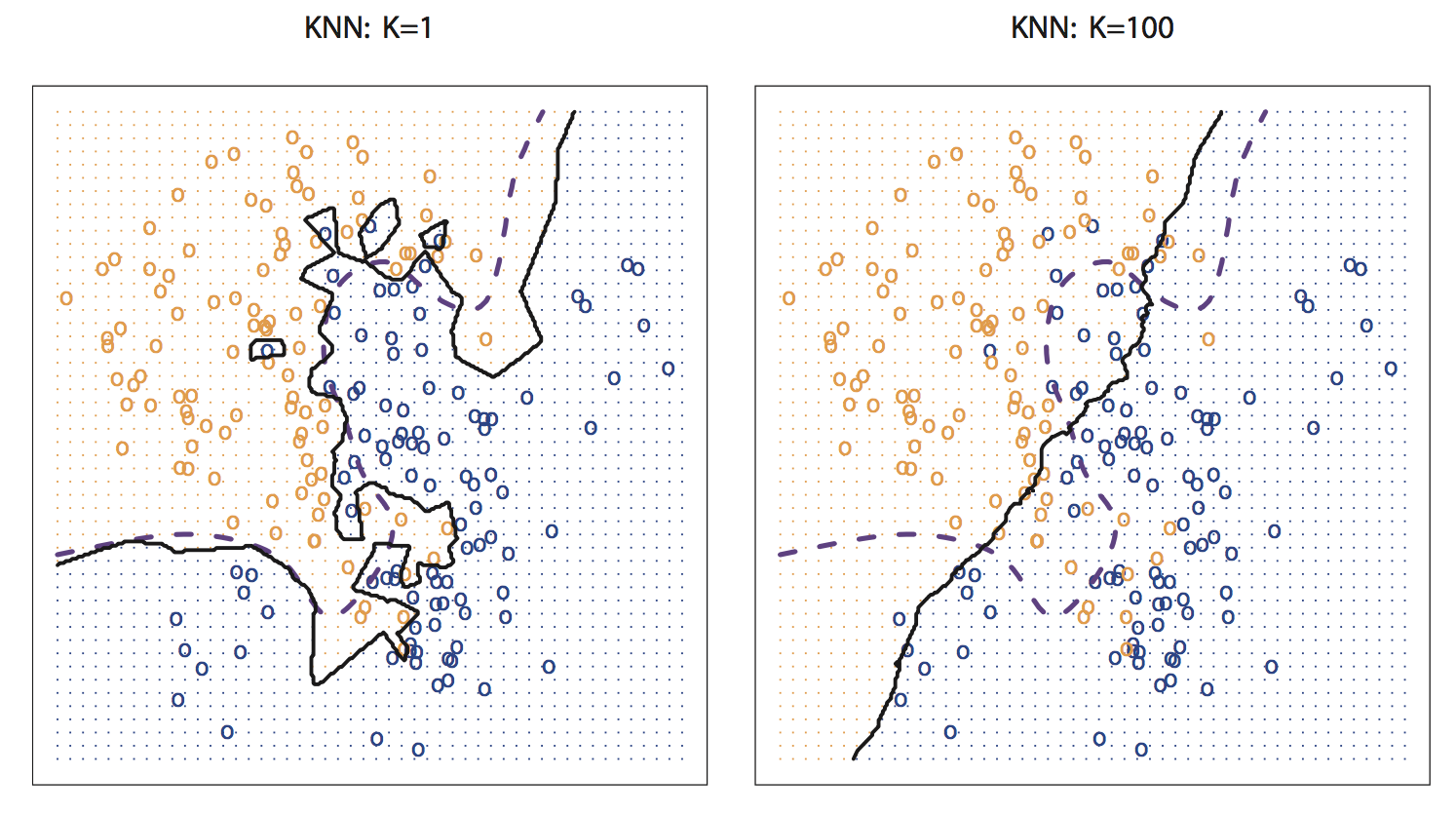
Model flexibility vs interpretability
From ISLR

Generalized additive models (GAMs)
- Relationships between individual predictors and the response are smooth
- Estimate the smooth relationships simultaneously to predict the response by adding them up

- GAMs have the advantage over GLMs of greater flexibility
A disadvantage of GAMs and other smoothing methods, compared with GLMs, is the loss of simple interpretability
How do we interpret the effect of a predictor on the response?
How do we obtain confidence intervals for those effects?
Generalized additive models (GAMs)

Smoothing splines
Goal: Estimate the smoothing spline \(\hat{s}(x)\) that balances the tradeoff between the model fit and wiggliness
Remember: Goldilocks principle

Predicting HRs with launch angle and exit velocity
HRs are relatively rare and confined to one area of this plot
batted_balls |>
  ggplot(aes(x = launch_speed,
             y = launch_angle,
             color = as.factor(is_hr))) +
  geom_point(alpha = 0.2)
Predicting HRs with launch angle and exit velocity
There is a sweet spot of launch_angle (mid-way ish) and launch_speed (relatively high) where almost all HRs occur
batted_balls |>
  group_by(
    launch_angle_bucket = round(launch_angle * 2, -1) / 2,
    launch_speed_bucket = round(launch_speed * 2, -1) / 2
  ) |>
  summarize(hr = sum(is_hr == 1),
            n = n()) |>
  ungroup() |>
  mutate(pct_hr = hr / n) |>
  ggplot(aes(x = launch_speed_bucket,
             y = launch_angle_bucket,
             fill = pct_hr)) +
  geom_tile() +
  scale_fill_gradient2(labels = scales::percent_format(),
                       low = "blue",
                       high = "red",
                       midpoint = 0.2)
Visualize partial response functions
Display the partial effect of each term in the model \(\longrightarrow\) add up to the overall prediction
library(gratia)
draw(hr_gam)
Convert to probability scale
Centered on average value of 0.5 because it’s the partial effect without the intercept
draw(hr_gam, fun = plogis)
Include intercept in plot
Intercept reflects relatively rare occurence of HRs
draw(hr_gam, fun = plogis, constant = coef(hr_gam)[1])
Model diagnostics
appraise(hr_gam)
Model checking
Check whether more basis functions are needed with gam.check() based on an approximate test
gam.check(hr_gam)
Method: REML   Optimizer: outer newton
full convergence after 9 iterations.
Gradient range [-1.611342e-05,4.419327e-06]
(score 627.7034 & scale 1).
Hessian positive definite, eigenvalue range [1.611218e-05,1.116216].
Model rank =  19 / 19

Basis dimension (k) checking results. Low p-value (k-index<1) may
indicate that k is too low, especially if edf is close to k'.

                  k'  edf k-index p-value
s(launch_speed) 9.00 1.00    0.97   0.095 .
s(launch_angle) 9.00 3.92    0.99   0.590
---
Signif. codes:  0 '***' 0.001 '**' 0.01 '*' 0.05 '.' 0.1 ' ' 1
Continuous interactions as a smooth surface
hr_gam_mult <- gam(is_hr ~ s(launch_speed, launch_angle), family = binomial, data = train)Plot the predicted heatmap (response on the log-odds scale)
# draw(hr_gam_mult)
hr_gam_mult |>
  smooth_estimates() |>
  ggplot(aes(launch_speed, launch_angle, z = .estimate)) +
  geom_contour_filled()
Continuous interactions as a smooth surface
Plot the predicted heatmap (response on the probability scale)
hr_gam_mult |>
  smooth_estimates() |>
  mutate(prob = plogis(.estimate)) |>
  ggplot(aes(launch_speed, launch_angle, z = prob)) +
  geom_contour_filled()